Sunday, June 13, 2021

ReLU

ReLU

2019/06/17

-----


Fig. ReLU(圖片來源)。

-----

References

A Practical Guide to ReLU – TinyMind – Medium
https://medium.com/tinymind/a-practical-guide-to-relu-b83ca804f1f7

Neural Networks  an Alternative to ReLU – Towards Data Science
https://towardsdatascience.com/neural-networks-an-alternative-to-relu-2e75ddaef95c

What is the 'dying ReLU' problem in neural networks  - Quora
https://www.quora.com/What-is-the-dying-ReLU-problem-in-neural-networks

'Dead ReLU Problem' 产生的原因 - Programming is an art form. - CSDN博客
https://blog.csdn.net/disiwei1012/article/details/79204243

Weight Decay

Weight Decay

2019/05/27

-----

References

Understanding the scaling of L² regularization in the context of neural networks
https://towardsdatascience.com/understanding-the-scaling-of-l%C2%B2-regularization-in-the-context-of-neural-networks-e3d25f8b50db

Monday, June 07, 2021

The Complete Stories of Jin Yong

The Complete Stories of Jin Yong

2019/05/27

-----


https://pixabay.com/zh/photos/classroom-school-education-learning-2093744/

-----

射雕三部曲


射雕

(56) 射鵰英雄傳之鐵血丹心 (粵語中字) 第一集 01/19 (黃日華,翁美玲 主演; TVB/1983) - YouTube

https://www.youtube.com/watch?v=YdOwu2l66nc&list=PLUxlohmoXranIaZNejFbL_lDUO6d-Rbtt


(57) 射鵰英雄傳之東邪西毒 (粵語中字) 01/20 (黃日華,翁美玲 主演; TVB/1983) - YouTube

https://www.youtube.com/watch?v=FlxU-VGePfs&list=PLUxlohmoXranyEYRPJjRvUIN8y7hxOchp


(57) 射鵰英雄傳之華山論劍 (粵語中字) 第一集 01/20 (黃日華,翁美玲 主演; TVB/1983) - YouTube

https://www.youtube.com/watch?v=ehnczdaDfm0&list=PLUxlohmoXralQp_KOzsfgqwhLMd60IZYX


神雕

(57) 神鵰俠侶 第一集 01/50 (劉德華,陳玉蓮 主演; TVB/1983) (粵語中字) - YouTube

https://www.youtube.com/watch?v=ZRznA7uSCB4&list=PLUxlohmoXram8z91p5ziJAwcoYhWHimpH


倚天

(59) 倚天屠龍記 01/40 | 梁朝偉、黎美嫻、鄧萃雯、邵美琪、鄭裕玲、任達華 | 粵語中字 | TVB 1986 - YouTube

https://www.youtube.com/watch?v=ZITWFwsfomg&list=PLYmVc4NVzaTy-mQCms5p4mhS7x1f-lVYu&index=1&t=161s

-----

天龍

(59) 天龍八部 01/45 | 黃日華、陳浩民、樊少皇、李若彤、趙學而、劉玉翠、劉錦玲 | 粵語中字 | TVB 1997 - YouTube

https://www.youtube.com/watch?v=1-_fKHpkfUE&list=PLUxlohmoXramdrlPfBj5P67YDrsxtYmws

-----

鹿鼎

(57) 鹿鼎記 01/40 | 梁朝偉、劉德華、劉嘉玲、毛舜筠、商天娥 | 粵語中字 | TVB 1984 - YouTube

https://www.youtube.com/watch?v=--UZ7qRYmQc&list=PLUxlohmoXramyQHliplHTl74OvARa2E1T

-----


References

[1] 金庸 - 維基百科,自由的百科全書
https://zh.wikipedia.org/wiki/%E9%87%91%E5%BA%B8

[2] 武俠小說- 好讀
http://www.haodoo.net/?M=hd&P=martial

[3] 读金庸的武侠小说,要留个心眼
http://www.sohu.com/a/272459386_482133 

Sunday, June 06, 2021

FCN(四):Appendix

 FCN(四):Appendix

2021/06/03

-----


# Focal Loss

說明:


-----


Table 4. Results on NYUDv2. RGBD is early-fusion of the RGB and depth channels at the input. HHA is the depth embedding of [13] as horizontal disparity, height above ground, and the angle of the local surface normal with the inferred gravity direction. RGB-HHA is the jointly trained late fusion model that sums RGB and HHA predictions.

表4. NYUDv2 上的結果。 RGBD 是輸入端的 RGB 和深度通道的早期融合。 HHA 是 [13] 的深度嵌入,包括水平差異,離地面的高度以及局部表面法線與推斷重力方向的夾角。 RGB-HHA 是聯合訓練的後期融合模型,將 RGB 和 HHA 預測相加。

說明:

略。

-----


Table 5. Results on SIFT Flow9 with class segmentation (center) and geometric segmentation (right). Tighe [33] is a non-parametric transfer method. Tighe 1 is an exemplar SVM while 2 is SVM + MRF. Farabet is a multi-scale convnet trained on class-balanced samples (1) or natural frequency samples (2). Pinheiro is a multi-scale, recurrent convnet, denoted RCNN3 (o3). The metric for geometry is pixel accuracy.

表5. SIFT Flow9 上具有類分割(中心)和幾何分割(右)的結果。 Tighe [33] 是一種非參數傳遞方法。 Tighe 1 是範例 SVM,而 2 是 SVM + MRF。 Farabet 是在類平衡樣本(1)或自然頻率樣本(2)上經過訓練的多尺度卷積網路。 Pinheiro 是一個多尺度的循環卷積網路,表示為 RCNN3(o 3)。 幾何指標是像素精度。

說明:

略。

-----

FCN(三):Illustrated

 FCN(三):Illustrated

2021/04/08

-----


https://pixabay.com/zh/vectors/network-iot-internet-of-things-782707/

-----


# ICNet

說明:

ICNet 在速度與正確性兩者間取得平衡。

-----


Figure 1. Fully convolutional networks can efficiently learn to make dense predictions for per-pixel tasks like semantic segmentation.

圖1. 全卷積網路可以有效地學習為每個像素任務(如語義分割)做出密集的預測。

# FCN

說明:

將最後一層熱圖經由 deconvolution 放大到原圖大小。實際上是 20 類加上背景 1 類。

最後 21 張熱圖,先透過 deconvolution 放大到原圖大小,然後 21 張的每個 xij 的點,最大值的點為預測類別。跟 groundtruth 比較後,可以知道預測是對還是不對。假設預測對的機率是 p,則使用 cross entropy loss(或其他)作為損失函數即可。

以此圖為例,訓練時 21 張特徵圖,有三張特徵圖,用貓狗背景當標籤。

-----


Figure 2. Transforming fully connected layers into convolution layers enables a classification net to output a heatmap. Adding layers and a spatial loss (as in Figure 1) produces an efficient machine for end-to-end dense learning.

圖2. 將全連接層轉換為卷積層使分類網能夠輸出熱圖。 增加層數和空間損失(如圖1 所示)將為端到端的密集學習提供一種高效的機器。

# FCN

說明:

將全連接層改成卷積層,則輸入不再需要固定大小。


以此圖為例,每張圖預測 1000 種類別,變成每個點預測 1000 種類別。同類別的點,集中成一張特徵圖。


如何決定一個點 xij 的類別?所有類別的特徵圖的 xij,最大值那張特徵圖的類別,即是 xij 預測的類別。

-----


# Focal Loss

說明:

Cross Entropy Loss,只要計算正確點的機率 p,的 - log( p ),即可。我們希望 p 越大越好,最好接近 1。p 越大,- log( p ) 越小(還是正值)。p = 1 時,Loss 為 0。

參考資料一


−(ylog(p)+(1−y)log(1−p))

Loss Functions — ML Glossary documentation

https://ml-cheatsheet.readthedocs.io/en/latest/loss_functions.html

參考資料二

損失函數|交叉熵損失函數- 知乎

https://zhuanlan.zhihu.com/p/35709485

參考資料三

https://blog.csdn.net/u014380165/article/details/77284921

參考資料四

https://eli.thegreenplace.net/2016/the-softmax-function-and-its-derivative/

-----


Figure 4.1: The transpose of convolving a 3 x 3 kernel over a 4 x 4 input using unit strides (i.e., i = 4, k = 3, s = 1 and p = 0). It is equivalent to convolving a 3 x 3 kernel over a 2 x 2 input padded with a 2 x 2 border of zeros using unit strides (i.e., i0 = 2, k0 = k, s0 = 1 and p0 = 2).

圖4.1:使用步幅將 3 x 3 內核卷積在 4 x 4 輸入上的轉置(即,i = 4,k = 3,s = 1 和 p = 0)。 這等效於使用單位步長(即 i0 = 2,k0 = k,s0 = 1 和 p0 = 2)在 2 x 2 輸入填充的 2 x 2 輸入上卷積 3 x 3 內核,並用零的 2 x 2 邊界填充。

# A Guide

說明:

先做 0 padding,然後用 3 x 3 的卷積核將 2 x 2 的圖放大到 4 x 4。

-----


Figure 3. Our DAG nets learn to combine coarse, high layer information with fine, low layer information. Pooling and prediction layers are shown as grids that reveal relative spatial coarseness, while intermediate layers are shown as vertical lines. First row (FCN-32s): Our singlestream net, described in Section 4.1, upsamples stride 32 predictions back to pixels in a single step. Second row (FCN-16s): Combining predictions from both the final layer and the pool4 layer, at stride 16, lets our net predict finer details, while retaining high-level semantic information. Third row (FCN-8s): Additional predictions from pool3, at stride 8, provide further precision.

圖3. 我們的 DAG 網路學習將粗糙的高層信息與精細的低層信息相結合。 池化層和預測層顯示為顯示相對空間粗糙度的網格,而中間層顯示為垂直線。 第一行(FCN-32s):如第 4.1 節所述,我們的單資料流網路將一步一步將步幅 32 的預測向上擴展至像素。 第二行(FCN-16):在步幅 16 結合來自最後一層和 pool4  層的預測,使我們的網路可以預測更精細的細節,同時保留高級語義信息。 第三行(FCN-8s):在步幅 8 中,來自 pool3 的其他預測提供了更高的精度。

說明:

FCN-32s 是將最後一層 deconv 32 倍。

FCN-16s 是將最後一層 deconv 2 倍,點對點相加,再 deconv 16 倍。較大的特徵圖要先預測,取出 21 張。

FCN-8s 是將最後一層 deconv 4 倍,點對點相加,再 deconv 8 倍。較大的特徵圖要先預測,取出 21 張。

-----


Table 1. We adapt and extend three classification convnets. We compare performance by mean intersection over union on the validation set of PASCAL VOC 2011 and by inference time (averaged over 20 trials for a 500 x 500 input on an NVIDIA Tesla K40c). We detail the architecture of the adapted nets with regard to dense prediction: number of parameter layers, receptive field size of output units, and the coarsest stride within the net. (These numbers give the best performance obtained at a fixed learning rate, not best performance possible.)

表1. 我們適應並擴展了三個分類卷積。 我們通過PASCAL VOC 2011 驗證集上的平均交集與並集以及推理時間(在 NVIDIA Tesla K40c 上進行 500 x 500 輸入的 20 多次試驗中得出的平均值)來比較性能。 我們針對密集預測詳細介紹了自適應網路的架構:參數層數,輸出單元的感受野大小以及網路內最粗的步幅。 (這些數字給出了以固定學習率獲得的最佳性能,而不是最佳性能。)

說明:

VGG16 效果最好。為何比 GoogLeNet 好?

rf size reception filter size

https://stackoverflow.com/questions/35582521/how-to-calculate-receptive-field-size

-----


Figure 4. Refining fully convolutional nets by fusing information from layers with different strides improves segmentation detail. The first three images show the output from our 32, 16, and 8 pixel stride nets (see Figure 3).

圖4. 通過融合來自具有不同跨度的圖層的信息來完善全卷積網路,可以改善分割細節。 前三個圖像顯示了我們 32、16 和 8 像素步幅網路的輸出(請參見圖3)。

說明:

FCN-32s 直接放大 32 倍。糊掉了。

-----


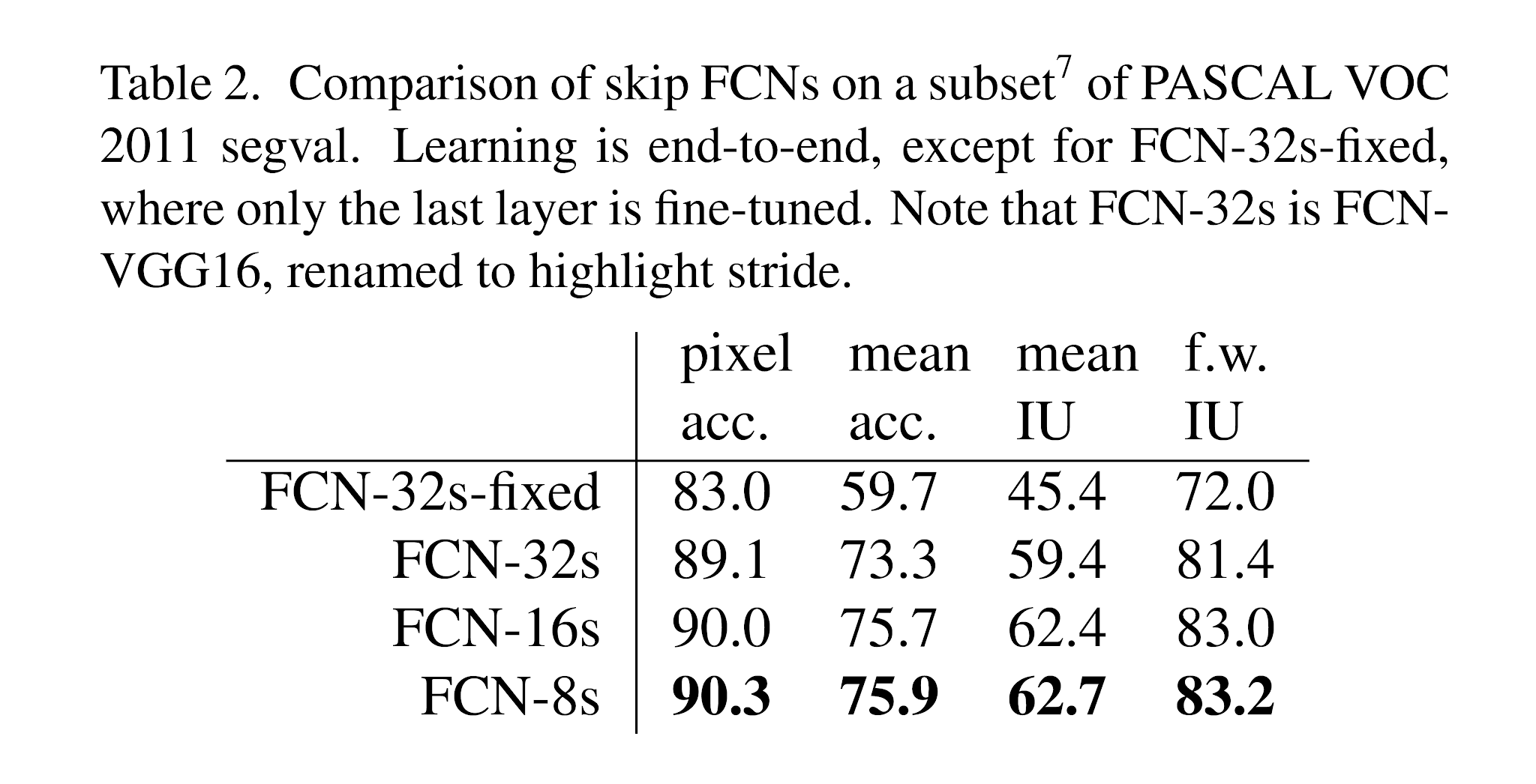
Table 2. Comparison of skip FCNs on a subset7 of PASCAL VOC 2011 segval. Learning is end-to-end, except for FCN-32s-fixed, where only the last layer is fine-tuned. Note that FCN-32s is FCN-VGG16, renamed to highlight stride.

表2. PASCAL VOC 2011 segval 的 subset7 上的跳過 FCN 的比較。 學習是端到端的,除了 FCN-32s 固定的(僅對最後一層進行微調)之外。 請注意,FCN-32 是 FCN-VGG16,已重命名以突出顯示步幅。

說明:

pixel accuracy 像素的正確率。

mean accuracy 類別準確率的平均。

mean IU(mIOU),IoU = TP / (TP + FP + FN)。 每類先算 IOU 再平均。

frequency weighted IU。根據每個類別出現的頻率設置權重。

https://medium.com/@chingi071/fully-convolutional-networks-%E8%AB%96%E6%96%87%E9%96%B1%E8%AE%80-246aa68ce4ad

-----


Figure 5. Training on whole images is just as effective as sampling patches, but results in faster (wall time) convergence by making more efficient use of data. Left shows the effect of sampling on convergence rate for a fixed expected batch size, while right plots the same by relative wall time.

圖5. 對整個圖像進行訓練與採樣色塊一樣有效,但是通過更有效地利用資料可以加快(牆上時間)收斂。 左圖顯示了對於固定的預期批次大小,採樣對收斂速度的影響,而右圖則通過相對牆上時間繪製了相同的結果。

說明:

取樣對批次次數無影響,但不取樣收斂時間較短,因為沒有重複的資料,比較有效率。

「wall time。這個很好理解,它就是我們從計算開始到計算結束等待的時間。除此之外,CPU time 也是一個常見的時間數據。CPU time 衡量的是 CPU 用來執行程序的時間。當軟件使用一個線程時,由於需要等待 IO 完成或者用戶輸入等原因,CPU 並不總是 100% 被使用,這導致CPU time 一般比 wall time 小。」

https://zhuanlan.zhihu.com/p/39891521

「如果 patchwise 的一個批處理剛好包含了價值函數所對整張圖接受,則相當於輸入整張圖像。但 patchwise 的方法卻每次每取一次批處理,總會有一些圖像塊是有重疊的。 輸入整張圖卻可以避免 patchbatch 之間的重疊,這樣更加高效。」。

https://www.daimajiaoliu.com/daima/6108d2427c9c805

-----


Table 3. Our fully convolutional net gives a 20% relative improvement over the state-of-the-art on the PASCAL VOC 2011 and 2012 test sets and reduces inference time.

表3. 我們的全卷積網路相對於 PASCAL VOC 2011 和 2012 測試集的最新技術提供了 20% 的相對改進,並減少了推理時間。

說明:

比 SDS 與 R-CNN 好。

-----


Figure 6. Fully convolutional segmentation nets produce stateof-the-art performance on PASCAL. The left column shows the output of our highest performing net, FCN-8s. The second shows the segmentations produced by the previous state-of-the-art system by Hariharan et al. [15]. Notice the fine structures recovered (first row), ability to separate closely interacting objects (second row), and robustness to occluders (third row). The fourth row shows a failure case: the net sees lifejackets in a boat as people.

圖6. 全卷積分割網在 PASCAL 上表現出最先進的性能。 左列顯示了性能最高的網路 FCN-8 的輸出。 第二部分顯示了 Hariharan 等人先前的最新系統所產生的分割結果,[15]。 注意恢復的精細結構(第一列),分離緊密相互作用的對象的能力(第二列)以及對遮擋物的穩健性(第三列)。 第四列顯示了一個失敗案例:網路將船上的救生衣視為人。

說明:

第一列,精細結構。

第二列,分離緊密的能力。

第三列,遮擋物。

救生衣認成人是 FCN 的缺點。SDS 為何不會?

-----


Fig. 1. U-net architecture (example for 32x32 pixels in the lowest resolution). Each blue box corresponds to a multi-channel feature map. The number of channels is denoted on top of the box. The x-y-size is provided at the lower left edge of the box. White boxes represent copied feature maps. The arrows denote the different operations.

圖1. U-net架構(最低分辨率的 32x32 像素範例)。 每個藍色框對應一個多通道特徵圖。 通道數顯示在框的頂部。 x-y 尺寸位於框的左下邊緣。 白框代表複製的特徵圖。 箭頭表示不同的操作。

說明:

黑色往右的箭頭。Conv3、ReLU。

灰色往右的箭頭。拷貝與裁減。

磚色往下的箭頭。max pooling 2 x 2。

綠色往上的箭頭。Deconv 2 x 2。

藍色往右的箭頭。Conv1。

虛線。裁減。

白框代表複製的特徵圖。

最後特徵圖為何有兩張?由於該任務是一個二分類任務,所以網路有兩個輸出 Feature Maps(背景與物件)。

損失函數此處不討論,可參考下方文章。

https://zhuanlan.zhihu.com/p/43927696

-----


Fig. 1.We improve DeepLabv3, which employs the spatial pyramid pooling module (a), with the encoder-decoder structure (b). The proposed model, DeepLabv3+, contains rich semantic information from the encoder module, while the detailed object boundaries are recovered by the simple yet effective decoder module. The encoder module allows us to extract features at an arbitrary resolution by applying atrous convolution.

圖1. 我們改進了 DeepLabv3,它使用了空間金字塔池模塊(a)和編碼器-解碼器結構(b)。 提出的模型 DeepLabv3 + 包含來自編碼器模塊的豐富語義信息,而詳細的對象邊界由簡單而有效的解碼器模塊恢復。 編碼器模塊允許我們通過應用空洞卷積以固定分辨率提取特徵。

說明:

spatial pyramid pooling 的部分為示意圖,細節可以參考圖 2。

-----


Fig. 2. Our proposed DeepLabv3+ extends DeepLabv3 by employing a encoderdecoder structure. The encoder module encodes multi-scale contextual information by applying atrous convolution at multiple scales, while the simple yet effective decoder module refines the segmentation results along object boundaries.

圖2。我們提出的 DeepLabv3 +通過採用編碼器/解碼器結構擴展了 DeepLabv3。 編碼器模塊通過在多個尺度上應用空洞卷積來編碼多尺度上下文資訊,而簡單而有效的解碼器模塊則沿著對象邊界細化分段結果。

說明:

Encoder 架構跟 Inception 類似。

-----


Fig. 3. 3×3 Depthwise separable convolution decomposes a standard convolution into (a) a depthwise convolution (applying a single filter for each input channel) and (b) a pointwise convolution (combining the outputs from depthwise convolution across channels). In this work, we explore atrous separable convolution where atrous convolution is adopted in the depthwise convolution, as shown in (c) with rate = 2.

圖3。3×3 深度可分離卷積將標準卷積分解為(a)深度卷積(對每個輸入通道應用單個濾波器)和(b)點向卷積(合併跨通道的深度卷積的輸出)。 在這項工作中,我們探索了空洞可分離卷積,其中在深度卷積中採用了空洞卷積,如(c)中所示,速率為 2。

說明:

a:一般卷積。

b:Conv1。

c:空洞卷積。或擴張卷積。

-----

# FCN

Long, Jonathan, Evan Shelhamer, and Trevor Darrell. "Fully convolutional networks for semantic segmentation." Proceedings of the IEEE conference on computer vision and pattern recognition. 2015.

https://www.cv-foundation.org/openaccess/content_cvpr_2015/papers/Long_Fully_Convolutional_Networks_2015_CVPR_paper.pdf


# Guide to convolution

Dumoulin, Vincent, and Francesco Visin. "A guide to convolution arithmetic for deep learning." arXiv preprint arXiv:1603.07285 (2016).

https://arxiv.org/pdf/1603.07285.pdf


# RetinaNet(Focal Loss)

Lin, Tsung-Yi, et al. "Focal loss for dense object detection." IEEE transactions on pattern analysis and machine intelligence (2018).

https://vision.cornell.edu/se3/wp-content/uploads/2017/09/focal_loss.pdf


# U-Net

Ronneberger, Olaf, Philipp Fischer, and Thomas Brox. "U-net: Convolutional networks for biomedical image segmentation." International Conference on Medical image computing and computer-assisted intervention. Springer, Cham, 2015.

https://arxiv.org/pdf/1505.04597.pdf


# DeepLab v3+

Chen, Liang-Chieh, et al. "Encoder-decoder with atrous separable convolution for semantic image segmentation." Proceedings of the European conference on computer vision (ECCV). 2018.

http://openaccess.thecvf.com/content_ECCV_2018/papers/Liang-Chieh_Chen_Encoder-Decoder_with_Atrous_ECCV_2018_paper.pdf


Multi-class cross entropy loss

https://www.oreilly.com/library/view/hands-on-convolutional-neural/9781789130331/7f34b72e-f571-49d2-a37a-4ed6f8011c93.xhtml


Review: FCN — Fully Convolutional Network (Semantic Segmentation) | by Sik-Ho Tsang | Towards Data Science

https://towardsdatascience.com/review-fcn-semantic-segmentation-eb8c9b50d2d1


FCN 的简单实现 - 知乎

https://zhuanlan.zhihu.com/p/32506912


FCN的学习及理解(Fully Convolutional Networks for Semantic Segmentation)_凹酱的DEEP LEARNING-CSDN博客_fcn

https://blog.csdn.net/qq_36269513/article/details/80420363


Fully Convolutional Networks 論文閱讀 | by 李謦伊 | May, 2021 | Medium

https://medium.com/@chingi071/fully-convolutional-networks-%E8%AB%96%E6%96%87%E9%96%B1%E8%AE%80-246aa68ce4ad


图像分割的U-Net系列方法 - 知乎

https://zhuanlan.zhihu.com/p/57530767


【U-Net】语义分割之U-Net详解 - 咖啡味儿的咖啡 - CSDN博客

https://blog.csdn.net/wangdongwei0/article/details/82393275


深入理解深度学习分割网络Unet——U-Net  Convolutional Networks for Biomedical Image Segmentation - 未来不再遥远 - CSDN博客

https://blog.csdn.net/Formlsl/article/details/80373200

-----

以下只列出論文

-----

# V-Net

Milletari, Fausto, Nassir Navab, and Seyed-Ahmad Ahmadi. "V-net: Fully convolutional neural networks for volumetric medical image segmentation." 2016 fourth international conference on 3D vision (3DV). IEEE, 2016.

https://arxiv.org/pdf/1606.04797.pdf


# 3D U-Net

Çiçek, Özgün, et al. "3D U-Net: learning dense volumetric segmentation from sparse annotation." International conference on medical image computing and computer-assisted intervention. Springer, Cham, 2016.

https://arxiv.org/pdf/1606.06650.pdf


# Deep Learning in Medical Image

Litjens, Geert, et al. "A survey on deep learning in medical image analysis." Medical image analysis 42 (2017): 60-88.

https://arxiv.org/pdf/1702.05747.pdf


# Skip Connections in Biomedical Image Segmentation

Drozdzal, Michal, et al. "The importance of skip connections in biomedical image segmentation." Deep Learning and Data Labeling for Medical Applications. Springer, Cham, 2016. 179-187.

https://arxiv.org/pdf/1608.04117.pdf


# Attention U-Net

Oktay, Ozan, et al. "Attention u-net: Learning where to look for the pancreas." arXiv preprint arXiv:1804.03999 (2018).

https://arxiv.org/pdf/1804.03999.pdf


# U-Net++

Zhou, Zongwei, et al. "Unet++: A nested u-net architecture for medical image segmentation." Deep Learning in Medical Image Analysis and Multimodal Learning for Clinical Decision Support. Springer, Cham, 2018. 3-11.

https://arxiv.org/pdf/1807.10165.pdf


MultiResUNet

Ibtehaz, Nabil, and M. Sohel Rahman. "MultiResUNet: Rethinking the U-Net architecture for multimodal biomedical image segmentation." Neural Networks 121 (2020): 74-87.

https://arxiv.org/pdf/1902.04049.pdf


DC-UNet

Lou, Ange, Shuyue Guan, and Murray Loew. "DC-UNet: Rethinking the U-Net Architecture with Dual Channel Efficient CNN for Medical Images Segmentation." arXiv preprint arXiv:2006.00414 (2020).

https://arxiv.org/ftp/arxiv/papers/2006/2006.00414.pdf

-----

FCN(二):Overview

FCN(二):Overview

2020/12/25

-----


https://pixabay.com/zh/photos/dog-cat-pets-animals-friends-2606759/

-----

◎ Abstract

-----

◎ Introduction

-----

本論文要解決(它之前研究)的(哪些)問題(弱點)? 

-----


# SDS。

-----

◎ Method

-----

解決方法? 

-----


# FCN

-----

具體細節?

https://hemingwang.blogspot.com/2021/04/fcnillustrated.html

-----

◎ Result

-----

本論文成果。 

-----

◎ Discussion

-----

本論文與其他論文(成果或方法)的比較。 

-----

成果比較。 

-----

方法比較。 

-----

◎ Conclusion 

-----

◎ Future Work

-----

後續相關領域的研究。 


# U-Net

-----

後續延伸領域的研究。


# Panoptic Segmentation。

-----

◎ References

-----

# SDS。被引用 983 次。

Hariharan, Bharath, et al. "Simultaneous detection and segmentation." European Conference on Computer Vision. Springer, Cham, 2014.

https://www2.eecs.berkeley.edu/Research/Projects/CS/vision/shape/papers/BharathECCV2014.pdf


# FCN。被引用 19356 次。

Long, Jonathan, Evan Shelhamer, and Trevor Darrell. "Fully convolutional networks for semantic segmentation." Proceedings of the IEEE conference on computer vision and pattern recognition. 2015.

https://www.cv-foundation.org/openaccess/content_cvpr_2015/papers/Long_Fully_Convolutional_Networks_2015_CVPR_paper.pdf


# Panoptic Segmentation

Kirillov, Alexander, et al. "Panoptic segmentation." Proceedings of the IEEE/CVF Conference on Computer Vision and Pattern Recognition. 2019.

https://openaccess.thecvf.com/content_CVPR_2019/papers/Kirillov_Panoptic_Segmentation_CVPR_2019_paper.pdf


# PFPNet。被引用 171 次。

Kirillov, Alexander, et al. "Panoptic feature pyramid networks." Proceedings of the IEEE Conference on Computer Vision and Pattern Recognition. 2019.

https://openaccess.thecvf.com/content_CVPR_2019/papers/Kirillov_Panoptic_Feature_Pyramid_Networks_CVPR_2019_paper.pdf


# Superpixel FCN

Yang, Fengting, et al. "Superpixel segmentation with fully convolutional networks." Proceedings of the IEEE/CVF Conference on Computer Vision and Pattern Recognition. 2020.

https://openaccess.thecvf.com/content_CVPR_2020/papers/Yang_Superpixel_Segmentation_With_Fully_Convolutional_Networks_CVPR_2020_paper.pdf


# II Superpixel FCN

Suzuki, Teppei. "Implicit Integration of Superpixel Segmentation into Fully Convolutional Networks." arXiv preprint arXiv:2103.03435 (2021).

https://arxiv.org/pdf/2103.03435.pdf

----- 

Tuesday, June 01, 2021

AI 從頭學(2021 年版)

AI 從頭學(2021 年版)

2020/01/01

全方位 AI 課程(精華篇)
http://hemingwang.blogspot.com/2020/01/all-round-ai-lectures-highlight.html

-----


Fig. 2021(圖片來源:Pixabay)。

-----

From Statistics to Deep Learning

-----


-----

What's the Main Points of Deep Learning?

-----


-----

一一、Regularization


一二、Normalization


一三、Optimization


一四、Activation Function


一五、Loss Function

-----

全方位 AI 課程(六十小時搞定深度學習)
https://hemingwang.blogspot.com/2020/01/all-round-ai-lectures.html

全方位 AI 課程(介紹篇)
https://hemingwang.blogspot.com/2020/01/all-round-ai-lectures-introduction.html

AI Seminar 2020 Taipei
https://hemingwang.blogspot.com/2019/12/ai-seminar-2020-taipei.html

-----

Python
https://hemingwang.blogspot.com/2019/02/python.html

-----

Part I:Computer Vision

◎ Image Classification

Stage 01:LeNet、(AlexNet、ZFNet)

Stage 02:NIN、(SENet、GoogLeNet、VGGNet、PreVGGNet、Highway v1 v2)、(Inception v3 v4、PolyNet)

Stage 03:ResNet v1 v2、(ResNet-D、ResNet-E、ResNet-I、ResNet-Q、ResNet-S、ResNet-W、WRN、ResNeXt、DenseNet、DPN、DLA、Res2Net)

◎ Semantic Segmentation

Stage 04:FCN、(DeconvNet、SegNet、U-Net、U-Net++、DilatedNet、ENet、DRN、FC-CRF、DeepLab v1 v2 v3 v3+、ResNet-38、RefineNet、RefineNet-LW、RefineNet-AA、PSPNet、ICNet、BiSeNet、Fast-SCNN、BlitzNet)

◎ Object Detection

Stage 05:(DPM、SS、R-CNN、SPPNet、Fast R-CNN、OHEM、Faster R-CNN、OverFeat)、YOLOv1、(SSD、DSSD、YOLOv2、ION、R-FCN、SATO、DCNv1、DCNv2、Cascade R-CNN、FPN、STDN、YOLOv3、RON、RefineDet、M2Det、DetNet、TridentNet、OHEM、Focal Loss、GHM、Libra R-CNN、DCRv1、DCRv2、PISA)

// ◎ Dataset

-----

Part II:Natural Language Processing

◎ LSTM
Stage 06:LSTM、(NNLM、Word2vec)

◎ Seq2seq
Stage 07:Seq2seq、(GloVe、fastText)

◎ Attention
Stage 08:Attention、(NTM、KVMN)

◎ ConvS2S
Stage 09:ConvS2S、(ELMo、ULMFiT)

◎ Transformer
Stage 10:Transformer、(GPT-1、BERT、GPT-2)

----- 

Part III:Fundamental Topics

◎ Regularization
Stage 11:(Weight Decay、L2、L1、L0、Dropout、DropConnect、DropPath、Scheduled DropPath、Shake-Shake、ShakeDrop、Spatial Dropout、Cutout、DropBlock、Fast Dropout、RNN Regularization、Variational Dropout、Information Dropout、DropEmbedding、Recurrent Dropout、Zoneout、AWD-LSTM、DropAttention、Mixup、Pairing Samples、AutoAugment)

◎ Normalization
Stage 12:(Batch、Weight、Layer、Instance、Group、Positional)

◎ Optimization
Stage 13:(SGD、Momentum、NAG、AdaGrad、AdaDelta、RMSProp、Adam、AdaMax、Nadam、AMSGrad、Lookahead、RAdam、LAMB、CLR、SGDR、AdamW、Super-Convergence、ADMM、ADMM-S、dlADMM)

◎ Activation Function
Stage 14:(sigmoid、tanh、ReLU、Softplus、LReLU、PReLU、ELU、SELU、GELU、Swish)

◎ Loss Function
Stage 15:

// ◎ Pooling
// ◎ Convolution
// ◎ Automatic Differentiation
// ◎ Back Propagation
// ◎ Computational Graph

-----

Part IV:Advanced Topics

◎ Instance Segmentation
Stage16:(Hypercolumn、MNC、DeepMask、SharpMask、MultiPathNet、InstanceFCN、FCIS)、Mask R-CNN、(MaskX R-CNN、MaskLab、PANet、HTC、RetinaMask、MS R-CNN、YOLACT)

◎ Mobile
Stage17:SqueezeNet、(MobileNet v1 v2 v3、ShuffleNet v1 v2、Xception)

◎ NAS
Stage18:NAS-RL、NASNet(Scheduled DropPath)、EfficientNet、Auto-DeepLab、NAS-FPN、 AutoAugment。

◎ GAN
Stage19:

◎ BERT
Stage20:

-----

Intelligence Science

-----

Intelligence Science
http://hemingwang.blogspot.com/2019/09/intelligence-science.html

-----


Part I:Computer Vision

-----

Computer Vision
https://hemingwang.blogspot.com/2019/10/computer-vision.html

https://hemingwang.blogspot.com/2019/10/gaussiansmooth.html

https://hemingwang.blogspot.com/2019/10/sobeledgedetection.html

https://hemingwang.blogspot.com/2019/10/structuretensor.html

https://hemingwang.blogspot.com/2019/10/nms.html

-----

◎ Image Classification

-----

Image Classification
https://hemingwang.blogspot.com/2019/10/image-classification.html

-----

◎ 1. LeNet(Image Classification)

-----

LeNet
https://hemingwang.blogspot.com/2019/05/trilogy.html
http://hemingwang.blogspot.com/2018/02/deep-learninglenet-bp.html
http://hemingwang.blogspot.com/2017/03/ailenet.html
http://hemingwang.blogspot.com/2017/03/ailenet-f6.html

AlexNet
http://hemingwang.blogspot.com/2017/05/aialexnet.html

PreAlexNet

ZFNet
http://hemingwang.blogspot.com/2017/05/aikernel-visualizing.html

PreZFNet

Deconv

-----

◎ 2. NINImage Classification)

-----

NIN
http://hemingwang.blogspot.com/2017/06/ainetwork-in-network.html

SENet
https://hemingwang.blogspot.com/2019/10/senet.html

SKNet
https://hemingwang.blogspot.com/2020/08/sknet.html

STNet
http://hemingwang.blogspot.com/2020/04/stnet.html

RANet

BAM

CBAM

RASNet

GoogLeNet
http://hemingwang.blogspot.com/2017/06/aigooglenet.html
http://hemingwang.blogspot.com/2017/06/aiconv1.html
http://hemingwang.blogspot.com/2017/08/aiinception.html

VGGNet
http://hemingwang.blogspot.com/2018/09/aivggnet.html 

PreVGGNet
https://hemingwang.blogspot.com/2019/11/prevggnet.html

Highway v1
http://hemingwang.blogspot.com/2019/11/highway.html

Highway v2

Inception v3
https://hemingwang.blogspot.com/2019/11/inception-v3.html

Inception v4
https://hemingwang.blogspot.com/2019/11/inception-v4.html

CapsNet v0

CapsNet v1
https://hemingwang.blogspot.com/2019/12/capsnet.html

CapsNet v2

CapsNet v3

-----

◎ 3. ResNetImage Classification)

-----

ResNet
https://hemingwang.blogspot.com/2019/05/vanishing-gradient.html
https://hemingwang.blogspot.com/2019/05/exploding-gradient.html
http://hemingwang.blogspot.com/2019/10/an-overview-of-resnet-and-its-variants.html
https://hemingwang.blogspot.com/2019/10/universal-approximation-theorem.html 
https://hemingwang.blogspot.com/2019/10/understanding-boxplots.html
https://hemingwang.blogspot.com/2019/10/ensemble-learning.html
http://hemingwang.blogspot.com/2018/09/airesnet.html


ResNet v1

ResNet-D
https://hemingwang.blogspot.com/2019/11/resnet-d.html

ResNet v2

ResNet-E
https://hemingwang.blogspot.com/2019/11/resnet-e.html

ResNet-V
https://hemingwang.blogspot.com/2019/12/resnet-v.html

-----

ResNet-F
https://hemingwang.blogspot.com/2019/12/resnet-f.html

ResNet-I
https://hemingwang.blogspot.com/2019/12/resnet-i.html

ResNet-Q
https://hemingwang.blogspot.com/2019/12/resnet-q.html

ResNet-S
https://hemingwang.blogspot.com/2019/11/resnet-s.html

ResNet-U
https://hemingwang.blogspot.com/2019/12/resnet-u.html 

ResNet-W
https://hemingwang.blogspot.com/2019/12/resnet-w.html

WRN
https://hemingwang.blogspot.com/2019/11/wrn.html

ResNeXt
https://hemingwang.blogspot.com/2019/10/resnext.html

DenseNet
https://hemingwang.blogspot.com/2019/11/densenet.html

DPN
https://hemingwang.blogspot.com/2019/11/dpn.html

DLA
https://hemingwang.blogspot.com/2019/11/dla.html

Res2Net
https://hemingwang.blogspot.com/2019/11/res2net.html

-----

PolyNet
https://hemingwang.blogspot.com/2019/11/polynet.html

FractalNet
https://hemingwang.blogspot.com/2019/12/fractalnet.html

RevNet

----- 

◎ 3.1. SqueezeNetImage Classification - Mobile)

-----

Mobile
https://hemingwang.blogspot.com/2019/10/mobile.html

SqueezeNet
https://hemingwang.blogspot.com/2019/10/squeezenet.html

MobileNet v1
https://hemingwang.blogspot.com/2019/10/mobilenet-v1.html

ShuffleNet

Xception
https://hemingwang.blogspot.com/2019/10/xception.html

-----

NAS-RL
https://hemingwang.blogspot.com/2019/12/nas-rl.html 

NASNet(Scheduled DropPath)
https://hemingwang.blogspot.com/2019/12/scheduled-droppath.html

EfficientNet 
https://hemingwang.blogspot.com/2019/12/efficientnet.html

Auto-DeepLab
https://hemingwang.blogspot.com/2019/12/auto-deeplab.html

NAS-FPN
https://hemingwang.blogspot.com/2019/12/nas-fpn.html 

AutoAugment
http://hemingwang.blogspot.com/2019/12/autoaugment.html

-----

◎ 4.1. FCN(Semantic  Segmentation)

-----

https://hemingwang.blogspot.com/2020/08/semantic-segmentation.html

-----

◎ 4.2. Instance Segmentation

-----

https://hemingwang.blogspot.com/2020/08/instance-segmentation.html

-----

◎ 4.3. Panoptic Segmentation

-----

https://hemingwang.blogspot.com/2020/08/panoptic-segmentation.html

-----

◎ 5. YOLOv1(Object Detection)

-----
 
Object Detection
https://hemingwang.blogspot.com/2019/10/object-detection.html 

-----

一、求好

DPM、SS、R-CNN、
SPPNet、Fast R-CNN、
Faster R-CNN、

-----

二、求快

OverFeat、YOLOv1、SSD、DSSD、YOLOv2、

-----

三、求好求快

ION、R-FCN、SATO、DCNv1、DCNv2、Cascade R-CNN、
FPN、STDN、YOLOv3、RON、RefineDet、M2Det、
SNIP、SNIPER、AutoFocus、
DetNet、TridentNet、

四、HARD

OHEM、Focal Loss、GHM、
Libra R-CNN、DCRv1、DCRv2、
PISA。

-----

DPM
https://hemingwang.blogspot.com/2019/11/dpm.html

SS
https://hemingwang.blogspot.com/2019/11/ss.html

R-CNN
https://hemingwang.blogspot.com/2019/11/r-cnn.html

SPPNet
https://hemingwang.blogspot.com/2019/11/sppnet.html

Fast R-CNN
https://hemingwang.blogspot.com/2019/11/fast-r-cnn.html

Faster R-CNN
https://hemingwang.blogspot.com/2019/09/faster-r-cnn.html 

-----

OverFeat
https://hemingwang.blogspot.com/2019/11/overfeat.html

YOLOv1
http://hemingwang.blogspot.com/2018/04/deep-learningyolo-v1.html
http://hemingwang.blogspot.com/2018/04/machine-learning-conceptmean-average.html
http://hemingwang.blogspot.com/2018/04/machine-learning-conceptnon-maximum.html
https://hemingwang.blogspot.com/2019/11/yolo-v1.html

SSD
https://hemingwang.blogspot.com/2019/09/ssd.html 

DSSD
https://hemingwang.blogspot.com/2019/11/dssd.html 

YOLOv2
https://hemingwang.blogspot.com/2019/11/yolo-v2.html

-----

ION
https://hemingwang.blogspot.com/2019/11/ion.html

R-FCN
https://hemingwang.blogspot.com/2019/11/r-fcn.html

SATO
https://hemingwang.blogspot.com/2019/10/sato.html 

DCNv1
https://hemingwang.blogspot.com/2019/12/dcn-v1.html

DCNv2
https://hemingwang.blogspot.com/2019/12/dcn-v2.html

Cascade R-CNN
https://hemingwang.blogspot.com/2019/12/cascade-r-cnn.html

FPN
https://hemingwang.blogspot.com/2019/11/fpn.html

STDN
https://hemingwang.blogspot.com/2019/12/stdn.html

YOLOv3
https://hemingwang.blogspot.com/2019/11/yolo-v3.html

RON
https://hemingwang.blogspot.com/2019/12/ron.html

RefineDet
https://hemingwang.blogspot.com/2019/11/refinedet.html

M2Det
https://hemingwang.blogspot.com/2019/10/m2det.html

SNIP
https://hemingwang.blogspot.com/2019/12/snip.html 

SNIPER
https://hemingwang.blogspot.com/2019/12/sniper.html

AutoFocus
https://hemingwang.blogspot.com/2019/12/autofocus.html

DetNet
https://hemingwang.blogspot.com/2019/12/detnet.html

TridentNet
https://hemingwang.blogspot.com/2019/12/tridentnet.html

-----

OHEM
https://hemingwang.blogspot.com/2019/11/ohem.html

Focal Loss
https://hemingwang.blogspot.com/2019/10/retinanet.html

GHM
https://hemingwang.blogspot.com/2019/12/ghm.html

Libra R-CNN
https://hemingwang.blogspot.com/2019/12/libra-r-cnn.html

DCRv1
https://hemingwang.blogspot.com/2019/12/dcr-v1.html

DCRv2
https://hemingwang.blogspot.com/2019/12/dcr-v2.html

PISA
https://hemingwang.blogspot.com/2019/12/pisa.html

-----
 
Part II:Natural Language Processing
 
-----

◎ 6. LSTM(NLP)

-----

LSTM
http://hemingwang.blogspot.com/2019/09/understanding-lstm-networks.html
https://hemingwang.blogspot.com/2019/09/lstm.html

-----

◎ NNLM

-----

MLE
EM
STM
n-gram

NNLM
https://hemingwang.blogspot.com/2019/04/nnlm.html

C&W
https://hemingwang.blogspot.com/2020/07/c.html

RNNLM
https://hemingwang.blogspot.com/2020/07/rnnlm.html

-----

◎ Word2vec 

-----

Word2vec
https://hemingwang.blogspot.com/2019/04/word2vec.html

Word2vec v1:CBOW and Skip-gram
https://hemingwang.blogspot.com/2020/07/word2vec-v1.html

Word2vec v2:Hierarchical Softmax and Negative Sampling
https://hemingwang.blogspot.com/2020/07/word2vec-v2.html

Word2vec v3:Simplified Word2vec v1 and v2
https://hemingwang.blogspot.com/2020/08/word2vec-v3.html

LSA
https://hemingwang.blogspot.com/2020/07/lsa.html

GloVe
https://hemingwang.blogspot.com/2020/07/glove.html

fastText v1
https://hemingwang.blogspot.com/2020/07/fasttext-v1.html

fastText v2
https://hemingwang.blogspot.com/2020/07/fasttext-v2.html

WordRank
https://hemingwang.blogspot.com/2020/07/wordrank.html

-----

◎ 7. Seq2seq(NLP)

-----

Seq2seq
http://hemingwang.blogspot.com/2019/10/word-level-english-to-marathi-neural.html
https://hemingwang.blogspot.com/2019/09/seq2seq.html

RNN Encoder-Decoder 1
http://hemingwang.blogspot.com/2020/08/rnn-encoder-decoder-1.html

RNN Encoder-Decoder 2
http://hemingwang.blogspot.com/2020/08/rnn-encoder-decoder-2.html

Teacher Forcing 1
http://hemingwang.blogspot.com/2020/08/teacher-forcing.html

Beam Search
http://hemingwang.blogspot.com/2020/08/beam-search.html

Curriculum Learning
http://hemingwang.blogspot.com/2020/08/curriculum-learning.html

-----

BoW 1-gram

Paragraph2vec
https://hemingwang.blogspot.com/2020/08/paragraph2vec.html

B4SE

PSE

-----

Skip-Thought

Quick-Thought

InferSent

MILA SE

Google SE

-----

S3E

SASE

SBERT

RRSE

-----

◎ 8. Attention(NLP)

-----

Attention
http://hemingwang.blogspot.com/2019/10/attention-in-nlp.html
http://hemingwang.blogspot.com/2019/01/attention.html

Attention 1
https://hemingwang.blogspot.com/2020/08/attention-1.html

Visual Attention
https://hemingwang.blogspot.com/2020/08/visual-attention.html

Grad-CAM
https://hemingwang.blogspot.com/2020/08/grad-cam.html

Attention 2
https://hemingwang.blogspot.com/2020/08/attention-2.html

GNMT
https://hemingwang.blogspot.com/2020/08/gnmt.html

-----

NTM

DNC

One Shot MANN

SMA

INTM

-----

MN

DMN

EEMN

KVMN

PN

Set2set

One Shot MN

FSA

-----

◎ 9. ConvS2S(NLP)

-----

ConvS2S
http://hemingwang.blogspot.com/2019/10/understanding-incremental-decoding-in.html 
https://hemingwang.blogspot.com/2019/04/convs2s.html

Key-Value
http://hemingwang.blogspot.com/2019/09/key-value.html

-----

S3L

Context2vec
https://hemingwang.blogspot.com/2020/08/context2vec.html

CoVe

ELLM

ELMo
https://hemingwang.blogspot.com/2019/04/elmo.html

ULMFiT

MultiFiT

-----

◎ 10. Transformer(NLP)

-----

Transformer
http://hemingwang.blogspot.com/2019/10/the-illustrated-transformer.html 
http://hemingwang.blogspot.com/2019/01/transformer.html

GPT-1
https://hemingwang.blogspot.com/2020/01/gpt-1.html

GPT-2

GPT-3

Grover

BERT
https://hemingwang.blogspot.com/2019/01/bert.html

-----

Reformer

LSH

RevNet

Adafactor

-----

Longformer

Synthesizer

Linformer

-----

Part III:Fundamental Topics

-----

Hyper-parameters
https://hemingwang.blogspot.com/2020/09/hyper-parameters.html


-----

◎ 11. Regularization

-----

Regularization

-----

◎ 12. Normalization

-----

PCA
https://hemingwang.blogspot.com/2020/10/understanding-principal-components.html

Normalization
http://hemingwang.blogspot.com/2019/10/an-overview-of-normalization-methods-in.html
https://hemingwang.blogspot.com/2019/10/normalization.html

BN
http://hemingwang.blogspot.com/2019/12/bn.html 

WN
http://hemingwang.blogspot.com/2019/12/wn.html 

LN
http://hemingwang.blogspot.com/2019/12/ln.html 

IN
http://hemingwang.blogspot.com/2019/12/in.html 

AIN
https://hemingwang.blogspot.com/2019/12/ain.html

GN
http://hemingwang.blogspot.com/2019/12/gn.html

PN
http://hemingwang.blogspot.com/2019/12/pn.html

UBN
http://hemingwang.blogspot.com/2019/12/ubn.html 

TUBN
https://hemingwang.blogspot.com/2019/12/tubn.html

ResNet-V
https://hemingwang.blogspot.com/2019/12/resnet-v.html

BNHO
http://hemingwang.blogspot.com/2019/12/bnho.html

URBN
http://hemingwang.blogspot.com/2019/12/urbn.html

NormProp
https://hemingwang.blogspot.com/2019/12/normprop.html 

Efficient Backprop
https://hemingwang.blogspot.com/2019/12/efficient-backprop.html

Whitening
https://hemingwang.blogspot.com/2019/12/whitening.html

GWNN
https://hemingwang.blogspot.com/2019/12/gwnn.html

DBN
https://hemingwang.blogspot.com/2019/12/dbn.html

KN
https://hemingwang.blogspot.com/2019/12/kn.html

IterNorm
https://hemingwang.blogspot.com/2019/12/iternorm.html

-----

-----

◎ 13. Optimization

-----

Optimization(一階)
http://hemingwang.blogspot.com/2019/10/an-overview-of-gradient-descent.html
https://hemingwang.blogspot.com/2018/03/deep-learningoptimization.html
https://hemingwang.blogspot.com/2019/01/optimization.html


Optimization(一階與二階)
https://hemingwang.blogspot.com/2020/10/5-algorithms-to-train-neural-network.html
https://hemingwang.blogspot.com/2020/10/optimization.html

-----

一階:

SGD、Momentum、NAG、
AdaGrad、AdaDelta、RMSProp、
Adam、AdaMax、 Nadam、AMSGrad、
RAdam、SMA、Lookahead、EMA、
AdaBound、SWATS、

LAMB、
CLR、SGDR、AdamW、Super-Convergence、

二階:

1. Gradient Descent, Jacobian, and Hessian、Taylor series and Maclaurin series、
2. Newton's Method、Gauss-Newton Method(Gauss-Newton Matrix)、
3. Conjugate Gradient(Gradient Descent + Newton's Method)、
4. Quasi Newton(Template)、SR1、Broyden(Family)、DFA、BFGS、L-BFGS、
5. Levenberg-Marquardt Algorithm(Gradient Descent + Gauss-Newton Method)
6. Natural Gradient Method(Fisher Information Matrix)、

Sunday, May 30, 2021

DenseNet(四):Appendix

 DenseNet(四):Appendix

2021/04/27

-----


-----

以下只列出論文

-----

# DPN

Chen, Yunpeng, et al. "Dual path networks." Advances in Neural Information Processing Systems. 2017.

https://proceedings.neurips.cc/paper/2017/file/f7e0b956540676a129760a3eae309294-Paper.pdf


# DLA

Yu, Fisher, et al. "Deep layer aggregation." Proceedings of the IEEE Conference on Computer Vision and Pattern Recognition. 2018.

http://openaccess.thecvf.com/content_cvpr_2018/papers/Yu_Deep_Layer_Aggregation_CVPR_2018_paper.pdf

-----

以下只列出論文

-----


一 CapsNet v0 論文

Hinton, Geoffrey E., Alex Krizhevsky, and Sida D. Wang. "Transforming auto-encoders." International conference on artificial neural networks. Springer, Berlin, Heidelberg, 2011.

http://www.cs.toronto.edu/~fritz/absps/transauto6.pdf


二 CapsNet v1 論文

Sabour, Sara, Nicholas Frosst, and Geoffrey E. Hinton. "Dynamic routing between capsules." arXiv preprint arXiv:1710.09829 (2017).

http://papers.nips.cc/paper/6975-dynamic-routing-between-capsules


三 CapsNet v2 論文

Hinton, Geoffrey E., Sara Sabour, and Nicholas Frosst. "Matrix capsules with EM routing." International conference on learning representations. 2018.

https://openreview.net/forum?id=HJWLfGWRb&noteId=BkelcSxC47


四 CapsNet v3 論文

Kosiorek, Adam R., et al. "Stacked capsule autoencoders." arXiv preprint arXiv:1906.06818 (2019).

http://papers.nips.cc/paper/9684-stacked-capsule-autoencoders


# CapsNet v4(被引用次數非常少)

Smith, Lewis, et al. "Capsule Networks--A Probabilistic Perspective." arXiv preprint arXiv:2004.03553 (2020).

https://arxiv.org/pdf/2004.03553.pdf


# Set Transformer

Lee, Juho, et al. "Set transformer: A framework for attention-based permutation-invariant neural networks." International Conference on Machine Learning. PMLR, 2019.

http://proceedings.mlr.press/v97/lee19d/lee19d.pdf


# Caps SS

LaLonde, Rodney, and Ulas Bagci. "Capsules for object segmentation." arXiv preprint arXiv:1804.04241 (2018).

https://arxiv.org/pdf/1804.04241.pdf


# CapsuleGAN

Jaiswal, Ayush, et al. "Capsulegan: Generative adversarial capsule network." Proceedings of the European Conference on Computer Vision (ECCV) Workshops. 2018.

https://openaccess.thecvf.com/content_ECCVW_2018/papers/11131/Jaiswal_CapsuleGAN_Generative_Adversarial_Capsule_Network_ECCVW_2018_paper.pdf

-----

DenseNet(三):Illustrated

 DenseNet(三):Illustrated

2021/03/27

-----


https://pixabay.com/zh/photos/city-architecture-building-urban-5051196/

-----

DenseNet 的第一個重點是圖4,比較 DenseNet、DenseNet-C、DenseNet-B,以及 DenseNet-BC 的異同。特別是 DenseNet-B 與 DenseNet 的差異。

DenseNet 的第二個重點是圖5。可參考 https://www.tensorinfinity.com/paper_89.html

DenseNet 的第三個重點是 "Visualizing the loss landscape of neural nets."  的圖7。

Li, Hao, et al. "Visualizing the loss landscape of neural nets." Advances in Neural Information Processing Systems. 2018.

https://papers.nips.cc/paper/2018/file/a41b3bb3e6b050b6c9067c67f663b915-Paper.pdf

-----


# DenseNet

說明:

growth rate

k 為 growth rate,也就是每一層的輸出。每一層的輸出,也會當成後續所有層的輸入。一般的作法是每張特徵圖通過一個卷積核,變成一張新的特徵圖。本論文重點是 k0 張如何變成 k 張。可以參考 LeNet。

-----


# LeNet。

六張特徵圖到十六張特徵圖。

說明:

以 16 張的第 0 張為例,它以六張的前三張共用一個卷積核。

combined

How are the feature maps of all filters in a convolutional layer combined? What is the final output of the layer?

「The feature maps from one layer are used to create new feature maps in the next layer. Each feature map in this second layer is a combination of all the feature maps in the first layer. And the value of the feature map in the second layer, at any one pixel, is found by multiplying each feature in the first layer with a convolution kernel, with a different kernel for each feature map in the first layer. The responses are then summed, added to a bias term, and then modified by a simple non-linear operation.」

卷積層中所有濾波器的特徵圖如何組合? 該層的最終輸出是什麼?

一層中的特徵圖用於在下一層中創建新的特徵圖。 第二層中的每個特徵圖都是第一層中所有特徵圖的組合。 通過將第一層中的每個特徵乘以卷積核,並為第一層中的每個特徵圖使用不同的核,可以找到第二層中任意一個像素的特徵圖的值。 然後將響應求和,添加到偏差項,然後通過簡單的非線性運算進行修改。

https://www.quora.com/How-are-the-feature-maps-of-all-filters-in-a-convolutional-layer-combined-What-is-the-final-output-of-the-layer

-----


# Convolution Guide

說明:

卷積可以視為稀疏的全連接層。

-----


Figure 1: A 5-layer dense block with a growth rate of k = 4. Each layer takes all preceding feature-maps as input.

圖1:一個 5 層密集塊,增長率為 k = 4。每一層都將所有先前的特徵圖作為輸入。

# DenseNet

說明:

假定第一層的輸入是 k0 張特徵圖,第一層的輸出是 k 張特徵圖。後面每一層的輸出都是 k 張特徵圖。每一層的輸出都會成為之後每一層的輸入。

那麼,這 k 張是怎麼決定的?標準方法不是用 Conv1。DenseNet-B 用 Conv1。

-----


Figure 2: A deep DenseNet with three dense blocks. The layers between two adjacent blocks are referred to as transition layers and change feature-map sizes via convolution and pooling.

圖2:具有三個密集塊的深 DenseNet。 兩個相鄰塊之間的層稱為過渡層,並通過卷積和池化更改特徵圖大小。

# DenseNet

說明:

過渡層,並通過 1x1 卷積降維,用池化更改特徵圖大小。

-----


Table 1: DenseNet architectures for ImageNet. The growth rate for the first 3 networks is k = 32, and k = 48 for DenseNet-161. Note that each “conv” layer shown in the table corresponds the sequence BN-ReLU-Conv.

表1:用於 ImageNet 的 DenseNet 架構。 前三個網路的增長率是 k = 32,而對於 DenseNet-161,k = 48。 注意,表中顯示的每個 “ conv” 層對應於序列 BN-ReLU-Conv。

# DenseNet

說明:

每個 “ conv” 層對應於序列 BN-ReLU-Conv。這張圖是 DenseNet-B。

-----


# DenseNet

說明:

每層增加 k 張會讓總數越來越多。瓶頸層用 Conv1 強制讓輸入變成 4k 張。

-----


# DenseNet

說明:

過渡層可以用 Conv1 壓縮特徵圖張數。本論文設定壓縮成一半的張數。

-----


Table 2: Error rates (%) on CIFAR and SVHN datasets. k denotes network’s growth rate. Results that surpass all competing methods are bold and the overall best results are blue. “+” indicates standard data augmentation (translation and/or mirroring).  indicates results run by ourselves. All the results of DenseNets without data augmentation (C10, C100, SVHN) are obtained using Dropout. DenseNets achieve lower error rates while using fewer parameters than ResNet. Without data augmentation, DenseNet performs better by a large margin.

表2:CIFAR 和S VHN 資料集的錯誤率(%)。 k 表示網路的增長率。 超過所有競爭方法的結果都是粗體,總體最佳結果是藍色。 “ +”表示標準資料擴充(轉換和/或鏡像)。 表示結果由我們自己決定。 使用 Dropout 可獲得 DenseNets 的所有不進行資料擴充的結果(C10,C100,SVHN)。 與 ResNet 相比,DenseNets 使用更少的參數可實現更低的錯誤率。 如果沒有資料擴充,DenseNet的性能將大大提高。

# DenseNet

說明:

粗體表示比所有競爭者好。

藍色表示是所有的裡面最好的。

+ 表示資料擴充(左上左下右上右下中、水平翻轉)。

-----


Table 3: The top-1 and top-5 error rates on the ImageNet validation set, with single-crop (10-crop) testing.

表3:使用單幅(10幅)測試的 ImageNet 驗證集上的 top-1 和 top-5 錯誤率。

# DenseNet

說明:

深度很重要,但寬度(k)似乎更重要。

-----


Figure 3: Comparison of the DenseNets and ResNets top-1 error rates (single-crop testing) on the ImageNet validation dataset as a function of learned parameters (left) and FLOPs during test-time (right).

圖3:在 ImageNet 驗證資料集上 DenseNets 和 ResNets top-1錯誤率(單幅測試)的比較,作為測試期間學習的參數(左)和 FLOP 的函數(右)。

# DenseNet

說明:

參數與浮點數運算都優於 ResNet。

-----


Figure 4: Left: Comparison of the parameter efficiency on C10+ between DenseNet variations. Middle: Comparison of the parameter efficiency between DenseNet-BC and (pre-activation) ResNets. DenseNet-BC requires about 1/3 of the parameters as ResNet to achieve comparable accuracy. Right: Training and testing curves of the 1001-layer pre-activation ResNet [12] with more than 10M parameters and a 100-layer DenseNet with only 0.8M parameters.

圖4:左圖:DenseNet 變體之間 C10 + 上參數效率的比較。 中:對比 DenseNet-BC 和(激活前)ResNets 的參數效率。 DenseNet-BC 需要大約 1/3 的參數作為 ResNet 才能達到可比的精度。 右圖:參數超過 10M 的 1001 層預激活 ResNet  [12] 和參數僅為 0.8M 的 100 層D enseNet的 訓練和測試曲線。

# DenseNet

說明:

左。DenseNet-BC 最優。

中。效能一樣的 DenseNet-BC,參數是 ResNet 的三分之一。

右。參數量較少的 DenseNet-BC,泛化能力比 ResNet 好。原因有可能是 DenseNet 是更稠密的 ensemble?

-----


Figure 5: The average absolute filter weights of convolutional layers in a trained DenseNet. The color of pixel (s, ℓ) encodes the average L1 norm (normalized by number of input feature-maps) of the weights connecting convolutional layer s to ℓ within a dense block. Three columns highlighted by black rectangles correspond to two transition layers and the classification layer. The first row encodes weights connected to the input layer of the dense block.

圖5:經過訓練的 DenseNet 中卷積層的平均絕對濾波器權重。 像素的顏色(s,ℓ)編碼在密集塊內將捲積層 s 連接到 ℓ 的權重的平均 L1 範數(通過輸入特徵圖的數量歸一化)。 用黑色矩形突出顯示的三列對應於兩個過渡層和分類層。 第一行對連接到密集塊輸入層的權重進行編碼。

# DenseNet

說明:

紅色表示 strong use,藍色表示 almost no use。橫坐標是選定層,縱坐標是選定層之前一層。最右方與最上方是 transition layer。


從圖中可以得到以下結論:

a) 較早的層提取出的特徵部分仍可能被較深的層使用。

b) 即便是 Transition layer 也有可能使用到之前 Denseblock 中所有的層的特徵。

c) 第 2 與第 3 個 Denseblock 中的層對之前的 Transition layer 利用率非常低,這表示 transition layer 會輸出大量冗餘的特徵。這也為 DenseNet-BC 提供證據支持,也就是 Compression 之必要。

d) 最後一層的分類層,雖然使用了之前 Denseblock 中的多層訊息,但更偏向使用最後幾個feature maps 的特徵。這說明在網路最後幾層,某些 high-level 的特徵可能會被產生。


https://www.tensorinfinity.com/paper_89.html

-----


Figure 4: The loss surfaces of ResNet-110-noshort and DenseNet for CIFAR-10.

# ResNet-V。

說明:

ResNet-110-noshort 與 DenseNet。DenseNet 也是 ensemble?!

-----


Figure 2: A deep DenseNet with three dense blocks. The layers between two adjacent blocks are referred to as transition layers and change feature-map sizes via convolution and pooling.

圖2:具有三個密集塊的深 DenseNet。 兩個相鄰塊之間的層稱為過渡層,並通過卷積和池化更改特徵圖大小。

# DenseNet

說明:

過渡層,並通過 1x1 卷積降維,用池化更改特徵圖大小。

-----


Are we really seeing convexity? We are viewing the loss surface under a dramatic dimensionality reduction, and we need to be careful interpreting these plots. For this reason, we quantify the level of convexity in loss functions but computing the principle curvatures, which are simply eigenvalues of the Hessian. A truly convex function has no negative curvatures (the Hessian is positive semi-definite), while a non-convex function has negative curvatures.

我們真的看到凸面了嗎? 我們正在觀察維度急劇減小下的損失表面,我們需要仔細解釋這些圖。 因此,我們可以對損失函數中的凸度進行量化,但要計算主曲率,這僅僅是 Hessian 的特徵值。 真正的凸函數不具有負曲率(Hessian 為正半定),而非凸函數則具有負曲率。

說明:

Hessian 為正半定,則為凸函數(平滑)。

-----


https://zh.wikipedia.org/wiki/%E9%BB%91%E5%A1%9E%E7%9F%A9%E9%99%A3

說明:

Hessian。

-----


https://ccjou.wordpress.com/2013/01/10/%E5%8D%8A%E6%AD%A3%E5%AE%9A%E7%9F%A9%E9%99%A3%E7%9A%84%E5%88%A4%E5%88%A5%E6%96%B9%E6%B3%95/

-----


# Hessian

說明:

特徵值與特徵向量。

-----


Figure 7: For each point in the filter-normalized surface plots, we calculate the maximum and minimum eigenvalue of the Hessian, and map the ratio of these two.

圖7:對於濾波器歸一化曲面圖中的每個點,我們計算 Hessian 的最大和最小特徵值,並映射這兩個的比率。

# ResNet-V。

說明:

對於濾波器歸一化曲面圖中的每個點,我們計算 Hessian 的最大和最小特徵值,並映射這兩個的比率。

Hessian 為半正定的話,最小特徵值為 0。畫面是深藍色。表示是 convex。若否,則偏黃。

-----


Figure 2: Architecture comparison of different networks. (a) The residual network. (b) The densely connected network, where each layer can access the outputs of all previous micro-blocks. Here, a 1 x 1 convolutional layer (underlined) is added for consistency with the micro-block design in (a). (c) By sharing the first 1 x 1 connection of the same output across micro-blocks in (b), the densely connected network degenerates to a residual network. The dotted rectangular in (c) highlights the residual unit. (d) The proposed dual path architecture, DPN. (e) An equivalent form of (d) from the perspective of implementation, where the symbol “o” denotes a split operation, and “+” denotes element-wise addition.

圖2:不同網路的架構比較。 (a)殘差網。 (b)稠密網,其中每個層都可以存取所有先前的微型塊的輸出。 這裡,為了與(a)中的微塊設計保持一致,添加了一個 1 x 1卷積層(底線)。 (c)通過在(b)中的微塊之間共享相同輸出的前 1 x 1連接,稠密網退化為殘差網。 (c)中的虛線矩形突出顯示了殘差單位。 (d)擬議的雙路徑架構 DPN。 (e)從實現的角度來看,(d)的等效形式,其中符號“ o”表示拆分運算,而“ +”表示逐元素加法。

# DPN

a ResNet。

b DenseNet。

c 將 DenseNet 轉成殘差格式。

d DPN。

e 是 d 的等效形式。

-----


# CSPNet

說明:

部分進入 DenseBlock,部分跳過 DenseBlock。運算量因而減少。結果可能接近。

-----

# DenseNet

Huang, Gao, et al. "Densely connected convolutional networks." Proceedings of the IEEE conference on computer vision and pattern recognition. Vol. 1. No. 2. 2017.

http://openaccess.thecvf.com/content_cvpr_2017/papers/Huang_Densely_Connected_Convolutional_CVPR_2017_paper.pdf


# LeNet

LeCun, Yann, et al. "Gradient-based learning applied to document recognition." Proceedings of the IEEE 86.11 (1998): 2278-2324.

http://yann.lecun.com/exdb/publis/pdf/lecun-01a.pdf


# Hessian

Brown, David E. "The Hessian matrix: Eigenvalues, concavity, and curvature." BYU Idaho Department of Mathematics (2014).

https://www.iith.ac.in/~ashok/Maths_Lectures/TutorialB/Hessian_Examples.pdf


# ResNet-V。被引用 464 次。ensemble 促使損失函數平滑化,也因此好訓練。

Li, Hao, et al. "Visualizing the loss landscape of neural nets." Advances in Neural Information Processing Systems. 2018.

https://papers.nips.cc/paper/2018/file/a41b3bb3e6b050b6c9067c67f663b915-Paper.pdf


# DPN

Chen, Yunpeng, et al. "Dual path networks." Advances in Neural Information Processing Systems. 2017.

https://proceedings.neurips.cc/paper/2017/file/f7e0b956540676a129760a3eae309294-Paper.pdf


# CSPNet

Wang, Chien-Yao, et al. "CSPNet: A new backbone that can enhance learning capability of CNN." Proceedings of the IEEE/CVF conference on computer vision and pattern recognition workshops. 2020.

https://openaccess.thecvf.com/content_CVPRW_2020/papers/w28/Wang_CSPNet_A_New_Backbone_That_Can_Enhance_Learning_Capability_of_CVPRW_2020_paper.pdf


# Convolution Guide

Dumoulin, Vincent, and Francesco Visin. "A guide to convolution arithmetic for deep learning." arXiv preprint arXiv:1603.

https://arxiv.org/pdf/1603.07285.pdf

-----

[1] DenseNet:比ResNet更優的CNN模型- 知乎

https://zhuanlan.zhihu.com/p/37189203


[2] DenseNet詳解

https://www.tensorinfinity.com/paper_89.html


[3] [線性系統] 對角化 與 Eigenvalues and Eigenvectors

https://ch-hsieh.blogspot.com/2010/08/eigenvalues-and-eigenvectors.html\


[4] 半正定矩陣的判別方法 | 線代啟示錄

https://ccjou.wordpress.com/2013/01/10/%E5%8D%8A%E6%AD%A3%E5%AE%9A%E7%9F%A9%E9%99%A3%E7%9A%84%E5%88%A4%E5%88%A5%E6%96%B9%E6%B3%95/


[5] (51) 【蜻蜓点论文】Visualizing the Loss Landscape of Neural Nets - YouTube

https://www.youtube.com/watch?v=xVxMvoacWMw


[6] (52) Tom Goldstein: "What do neural loss surfaces look like?" - YouTube

https://www.youtube.com/watch?v=78vq6kgsTa8

-----

DenseNet - Keras

keras-applications/densenet.py at master · keras-team/keras-applications · GitHub

https://github.com/keras-team/keras-applications/blob/master/keras_applications/densenet.py


DenseNet - TensorFlow

GitHub - taki0112/Densenet-Tensorflow: Simple Tensorflow implementation of Densenet using Cifar10, MNIST

https://github.com/taki0112/Densenet-Tensorflow


DenseNet - PyTorch

vision/densenet.py at master · pytorch/vision · GitHub

https://github.com/pytorch/vision/blob/master/torchvision/models/densenet.py

-----