AI 從頭學(一二):LeNet
2017/03/01
前言:
關於 LeNet-5,寫完這篇,我給自己打 70 分勉強及格。
-----
Fig. Net(圖片來源:
Pixabay)。
-----
Summary:
LeNet-5 [1]-[2],是 Convolutional Neural Network (CNN) [3]-[8] 的基本應用。關於CNN,有網路上的投影片 [9]-[11]、論文章節 [12]-[15]、電子書章節 [16]-[18] 可供參考。
CNN 重要的計算,分別有 Convolution [19]-[20]、Activation function [21]、與 Sub-sampling [19]-[20]。有關 LeNet-CNN 的實作,可參考 Caffe [22]-[23]、TensorFlow [24]、Theano [25]-[26]、與Keras [27]。
CNN 是深度學習(目前幾乎是人工智慧的代名詞)的一支,主要,但不限於影像辨識。它的架構受到大腦視覺皮層研究的啟發 [28]-[35],由於近年來電腦軟硬體運算能力提升很多,因此蔚為風行。
-----
Hierarchy
C1 6@28x28, simple cells (edges)
S2 6@14x14
C3 16@10x10, complex cells (object parts, shapes)
S4 16@5x5
C5 (120@1x1)=8x15 (objects, topological)
F6 84=7x12 (physical)
F7 10 (abstract)
LeNet-5 共有七層,參考圖1a。在解說每層之前,先簡單介紹一下整體架構以便瞭解。
C1、C3、C5 是 convolution layer,主要是萃取影像的特徵。在生理上,「大約」可以對應到視覺皮層的 V1、V2、V4、IT 等構造,參考圖1b、1c。這個設計是受到生理學家做的實驗所啟發,在貓或猴子的初級視覺皮層置入電極,對不同方向的線條刺激,反應也有所不同,參考圖1d。
C1、C3、C5「大約」可以對應 simple cells、complex cells、以及 hypercomplex cells [32]-[34]。
S2、S4 主要都是縮小資料量。
最後 F6、F7 則是傳統的類神經網路。
Convolution 的層級不一定只有三,也可以更多。如果是三層,我們可以假定 C1 是偵測邊緣的線條,C3 偵測物體的局部,C5 偵測整個物體,參考圖1e。如果是四層,可以分成 edges、motifs、parts、objects [14] 。
-----
圖一:
Fig. 1a. LeNet-5 [1]。
Fig. 1b. Sketch of the Hmax hierarchical model of visual processing, p. 16, [35]。
Fig. 1c. The extrastriate cortex, p. 220, [30]。
Fig. 1d. Experiments of single neurones in the cat's striate cortex, p. 7, [11]。
Fig. 1e. Hierarchy of face recognition, p. 478 [16]。
-----
Q1:What do these numbers (Input: 32x32, C1: 6@28x28, S2: 6@14x14, C3: 16@10x10, S4: 16@5x5, C5: 120, F6: 84, Output: 10) mean?
Q2:What is sparse connectivity?
Q3:What are shared weights?
Q4:What is zero padding?
這邊還是採取自問自答的方式進行。
-----
Q1:What do these numbers (Input: 32x32, C1: 6@28x28, S2: 6@14x14, C3: 16@10x10, S4: 16@5x5, C5: 120, F6: 84, Output: 10) mean?
-----
A0_Input: 32x32
輸入層是 32x32 pixels 的圖片,為何是 32,這在論文中解釋的很清楚。因為原始圖片的大小是 28x28。32x32 做完 5x5 filters 的 convolution 後,影像,也就是 feature maps 的大小會變成 28x28,不致於有邊緣資料訊息的損失。細節請參考圖2g 與底下 zero padding 的說明。
-----
A1_C1: 6@28x28
32x32 的原始圖片經過六個 5x5 的 edge filters 後,變成六張 28x28 的圖片,這些圖片稱為 feature maps,因為這些圖是由不同角度的線條所組成。六是一個參考值,也可以設為八,如圖2a。Filters 也可以更複雜如圖2b、2c、2d。真實的 filters 長什麼樣,可以參考圖2e。
Convolution 的運算,在一維的空間,可以想成多項式相乘。概念推到二維,就是圖片跟 filter 的 convolution,詳細的運算式,可以參考 [19]-[20]。
做完 convolution 後,緊接著是 activation function,這在圖1a並沒有標示出來,可參考圖3a。主要的 activation functions 有 sigmoid 與 ReLU,見圖3b、3c。關於 activation functions 的介紹,請參考 [21]。
這邊對 C1 做個小結:32x32 的原始圖片,經過六個 5x5 的 edge detection filters 後,變成六張 28x28 的 feature maps,然後再做 activation operation。
值得注意的是 filters 的數目、大小,都是可調整的 [25]。Activation function 的選擇,則以ReLU 為佳 [21]。
-----
圖二:
Fig. 2a. Edge filters, [8]。
Fig. 2b. Cortical filter models of the primary visual cortex, p. 2, [35]。
Fig. 2c. Divisive normalization in the primary visual cortex, p. 5, [35]。
Fig. 2d. A computer emulation of "edge detection" using retinal receptive fields [31]。
Fig. 2e. Edge detection filter, p. 7, [9]。
Fig. 2f. Complicated filter, p. 15, [9]。
Fig. 2g. Filter size, input/output size, and zero padding, p. 12, [9]。
-----
圖三:
Fig. 3a. Non-linearity, [23]。
Fig. 3b. Sigmoid function, p. 475, [16]。
Fig. 3c. ReLU function, [5]。
-----
A2_S2: 6@14x14
S2 相對 C1 簡單不少。
六張 28x28 的 feature maps 做完 subsampling 後,得到六張 14x14 的feature maps。主要目的是減少資料量以便運算。方法是每 2x2 的方塊取一點。或者取最大的一點,或者是四點平均,叫做 pooling,參考圖4a。一樣,做 max-pooling 時,方塊大小也是可以調整的 [25]。
除了減少運算量,sub-sampling 還有許多好處,譬如避免 overfitting,參考圖4b,然而最新的趨勢是增加 convolutional layers 的層數,pooling 不做,參考圖4c。Overfitting,簡單說,就是做考古題時接近滿分,真的上考場表現卻大不如預期。
-----
圖四:
Fig. 4a. Sub-sampling, p. 19, [9]。
Fig. 4b. Advantages of pooling, [5]。
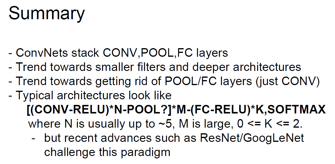
Fig. 4c. Trends of ConvNets, p. 89, [11]。
-----
A3_C3: 16@10x10
六個 14x14 的 feature maps 經過 C3 後,會變成十六個 10x10 的 feature maps。
Filters 的大小還是 5x5,所以 14x14 會變成 10x10。然後十六個 feature maps 是由六個中哪些得出,參考圖五,比方說,十六個中的第一個,由六個中的第一二三個分別做完 convolution 再組成。
參考圖1e跟2f,我們可以知道這一層要把線條組成局部的圖,以數字而言就是圓圈、半圓、折線、直線、十字等等。角度不要太大,所以要連續取好幾個。希望要有點變化,兩個太少,至少要三個。然後是連四。連二加連二已經接近連六。最後是連六,十字可能就由連六獲得。這段是由現有資料推論得來。
Convolution之後,還是 activation operation。
-----
圖五:
Fig. 5. Connections between S2 and C3, p. 8, [1]。
-----
A4_S4: 16@5x5
10x10 再經過 sub-sampling 之後,變成 5x5。
-----
A5_C5: 120
這一層其實是 16@5x5,經過 5x5 的 filters 後,變成 120@1x1。120 個點,就可以跟下一層的 84 個點做一個 full connection。
為什麼是 120 呢?這邊要大膽猜測一下,因為下一層是 7x12,所以這一層取 8x15,稍微大一點,可以看成是拓樸(形狀)上的 0 到 9。下一層是實體的 0 到 9,最後一層是抽象的 0 到 9。
參考圖2f、1e,這一層所有的點組合起來應該已經不是如圖2f 的局部,而是如圖1e 的最高層,是數字的形狀了。因為已經有三層 filters 了。
-----
A6_F6: 84
84,是 7x12 的 ASCII 字元,參考論文 [1]。
-----
A7_F7: 10
A7 這一層決定輸出是 0 到 9 哪一個數字,由前一層 7x12 個點計算 Euclidean Radial
Basis Function units (RBF) 。這一段我還是不很懂,只能說需要強調的點(w大)存在(x大),或者不需要強調的點(w小)不存在(x小),則 error 小。未來若有機會再另行補充。
A0 到 A7 分別 Answer了 Q1 這七層為何要如此設計。
-----
Q2:What is sparse connectivity?
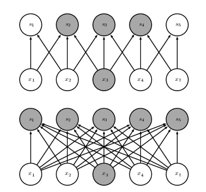
CNN在每兩層的連接,不一定要全部的點都連起來,參考圖6a、6b、6c。主要是利用 receptive fields 的特性:V1 上的 simple cells,只會對視網膜上的小塊區域的刺激有反應 [28]-[35]。V4 上的 complex cells,反應的範圍就很大。
所以 Sparse connectivity 一方面減少資料的運算,一方面有生理學的基礎,而實際的表現也很好。
-----
圖六:
Fig. 6a. Sparse connection, [25]。
Fig. 6b.
Sparse connectivity, viewed from below, p. 336, [3]。
Fig. 6b.
Sparse connectivity, viewed from above, p. 337, [3]。
Fig. 6c. The
receptive
field
of
the
units
in
the
deeper
layers
of
a
convolutional
network is
larger
than
the
receptive
field
of
the
units
in
the
shallow
layers, p. 337, [3]。
-----
Q3:What are shared weights ?
這邊我想先抄幾段參考資料的英文,然後再用中文簡單說明。
Weights of the same color are shared—constrained to be identical [25].
In a convolutional neural net, each member of the kernel is used at every position of the input (except perhaps some of the boundary pixels, depending on the design decisions regarding the boundary) [3].
The kernel moves along (and thus shared across) the input with strides (or subsampling rate) Sr and Sc at the vertical (row) and horizontal (column) direction, respectively [18].
Here, the key idea is that if a feature detector is useful in one part of the image, it might be useful in another part as well [17].
In other words, if a motif can appear in one part of the image, it could appear anywhere, hence the idea of units at different locations sharing the same weights and detecting the same pattern in different parts of the array [14].
Shared weights 其實是緊接著 sparse connectivity 而來,一個 spacial filter 掃過整張畫面,這個 filter 的值其實是不變的,譬如,對一張畫面要萃取橫條紋,就用同一個 filter,這不是理所當然嗎?參考圖7a、7b。
與 sparse connectivity 相同,shared weights 也減少運算量。
-----
圖七:
Fig. 7a. Weights sharing, [25]。
Fig. 7b. Weights sharing:
Blac
k
arrows
indicate
the
connections
that
use
a
particular parameter
in
tw
o
different
mo
dels, p. 338, [3]。
-----
Q4:What is zero padding?
由於 convolution 會讓圖越變越小,參考圖2g。若要避免,可以做 zero padding。也有不做 zero padding的例子 [19]。
-----
Jason Tsai:「補充一下,28x28 原圖擴展成 32x32 當作輸入是在原圖四邊補空白黑邊,稱為 zero padding,在這個辨識像這種小像素數字和英文字母的應用中,維持 C1 後仍為 28x28 的目的有二:1. 避免像素空間特徵的損失、2. 避免邊緣特徵的流失。在現在彩色大像素已事先 normalized 的圖片辨識中 zero padding 多用來微調輸入圖片大小以匹配 convolution 過程中的整數四則運算。」
-----
Conclusion:
即將寫完這篇,我想說,LeNet-5 在理解上不是太難,但設計的人可說是天才。天才不是一天造成的,也不是一個人憑空就會是天才,而是站在無數前人的努力上,更進一步。
在 LeNet 1998 之後,由於近年來硬體的運算提升,CNNs 又有更新的設計:AlexNet 2012、ZFNet 2013、GoogLeNet 2014、VGGNet 2014、ResNet 2015、DenseNet 2016
[5], [7], [11]。錯誤率繼續下降,而層數急速上升,參考圖8。而最新的趨勢,請參考圖4c。
最後,容我翻轉一下據說是貝多芬的遺言:諸君,喝采吧。喜劇已開場!
-----
圖八:
Fig. 8. Evolution of depth, p. 33, [10]。
-----
出版說明:
2019/09/23
1998 年,LeNet 奠定了 CNN 主要的架構:卷積層、池化層、全連接層。透過反向傳播法跟梯度下降法更新權重,成功辨識阿拉伯數字 0 到 9,並且應用在部分美國銀行的支票辨識系統上。
-----
References
◎ [1] 1998_Gradient-Based Learning Applied to Document Recognition
[2] Deep Learning(深度学习)学习笔记整理系列之LeNet-5卷积参数个人理解 - qiaofangjie的专栏 - 博客频道 - CSDN_NET
http://blog.csdn.net/zouxy09/article/details/8781543
◎ [3] 9 Convolutional Networks
http://www.deeplearningbook.org/contents/convnets.html
[4] Convolutional neural network – Wikipedia
https://en.wikipedia.org/wiki/Convolutional_neural_network
◎ [5] An Intuitive Explanation of Convolutional Neural Networks – the data science blog
https://ujjwalkarn.me/2016/08/11/intuitive-explanation-convnets/
[6] Convolutional Neural Networks (CNNs) An Illustrated Explanation – XRDSXRDS
http://xrds.acm.org/blog/2016/06/convolutional-neural-networks-cnns-illustrated-explanation/
[7] CS231n Convolutional Neural Networks for Visual Recognition
http://cs231n.github.io/convolutional-networks/
[8] [DL] Convolutional Neural Network ? 不要停止思考
http://solring-blog.logdown.com/posts/302641-dl-convolutional-neural-network
[9] 6_CNN.pdf
http://classes.engr.oregonstate.edu/eecs/winter2017/cs519-006/Slides/6_CNN.pdf
[10] Convnets.pdf
http://www.cs.toronto.edu/~guerzhoy/411/lec/W06/convnets.pdf
[11] winter1516_lecture.pdf
http://cs231n.stanford.edu/slides/winter1516_lecture7.pdf
[12] 2016_Towards Bayesian Deep Learning, A Survey_3-4
[13] 2016_Deep Learning on FPGAs, Past, Present, and Future_2-3
[14] 2015_Deep learning_4-5
[15] 2009_Learning deep architectures for AI_43-45
[16] 2016_Practical Machine Learning_493-495
[17] 2015_Python Machine Learning_381-383
[18] 2015_Automatic speech recognition, a deep learning approach_288-291
[19] 2015_A guide to convolution arithmetic for deep learning
◎ [20] 2002_Tutorial on Convolutions – Torch
◎ [21] Google軟件工程師解讀:深度學習的activation function哪家強?_幫趣網
http://bangqu.com/gpu/blog/5484
[22] Caffe LeNet MNIST Tutorial
http://caffe.berkeleyvision.org/gathered/examples/mnist.html
[23] LeNet CNN 實例 MNIST 手寫數字辨識 allenlu2007
https://allenlu2007.wordpress.com/2015/11/28/mnist-database-%E6%89%8B%E5%AF%AB%E6%95%B8%E5%AD%97%E8%BE%A8%E8%AD%98/
[24] Playing with convolutions in TensorFlow — Mourad Mourafiq
http://mourafiq.com/2016/08/10/playing-with-convolutions-in-tensorflow.html
◎ [25] Theano - Convolutional Neural Networks (LeNet) — DeepLearning 0_1 documentation
http://deeplearning.net/tutorial/lenet.html
[26] 卷积神经网络 Convolutional Neural Networks (LeNet) - Maching Vision - 博客园
http://www.cnblogs.com/cvision/p/CNN.html
[27] LeNet - Convolutional Neural Network in Python - PyImageSearch
http://www.pyimagesearch.com/2016/08/01/lenet-convolutional-neural-network-in-python/
[28] 1962_Receptive fields, binocular interaction, and functional architecture in the cat’s visual cortex
[29] 1968_Receptive fields and functional architecture of monkey striate cortex
◎ [30] 2016_Ocular and visual physiology, clinical application_201-228
[31] Receptive field – Wikipedia
https://en.wikipedia.org/wiki/Receptive_field
[32] Simple cell – Wikipedia
https://en.wikipedia.org/wiki/Simple_cell
[33] Complex cell – Wikipedia
https://en.wikipedia.org/wiki/Complex_cell
[34] Hypercomplex cell – Wikipedia
https://en.wikipedia.org/wiki/Hypercomplex_cell
◎ [35] 2017_Towards a theory of computation in the visual cortex