Monday, September 30, 2019

深入淺出 Deep Learning(二):LeNet & BP

深入淺出 Deep Learning(二):LeNet & BP

2018/02/23

前言:

我是讀懂 BP 後再仔細看 LeNet 的。經過幾次實際的講解,我想先講 LeNet 比較適合,所以更新順序,並增加了實例的部分,希望可以更清楚一些!

-----


Fig. The Net(圖片來源:PixaBay)。

-----

Summary:

深度學習 [1], [2] 的核心是 LeNet [3]。

本文從多項式 [4] 出發,詳細地解釋 LeNet [5], [6] 與 Back Propagation [7] 演算法,並指出權重是經由訓練而得這個重點 [8]。最後是 LeNet 的實作 [9] 與更多深度學習論文講解 [10]。

-----

Outline:

一、Introdunction
二、Polynomial
三、LeNet
四、Convolution
五、Activation Function
六、Pooling
七、Back Propagation

-----

一、Introdunction

一年多前,在我剛開始接觸 Deep Learning 的時候,那時 AlphaGo 早就以四勝一負的戰績擊敗韓國的李世石。不過真正引起我關注的是 chatbot:聊天機器人,如果你不深入 AI 的理論,只想呼叫現成的 APIs,那有什麼搞頭呢?

那時我拿到博士學位還沒很久,正規的訓練,要切入一門新領域,可以從集大成的論文開始,我找了幾篇 [1],並且看完其中最重要的 [2]。大體上這並沒有錯,不過真正的奧秘是你必須先精讀某篇論文 [3],這篇其實也藏在 [2] 裡面,不過沒人跟你講,你是很難發現的。

總之,當我不是很懂就開始發表心得時 [1],就有熱心人士來指導了。花了一些時間後,終於看懂了論文 [3] 裡面的 Back Propagation 演算法 [7],以及後續不計其數的論文 [10]。

一年過去了,我試著把這個題目重新寫一遍,看看是不是可以更簡明!

-----

二、Polynomial

LeNet 屬於類神經網路(Artificial Neural Networks, ANN)中的一種,中文叫做卷積神經網路(Convolutonal Neural Networks, CNN)。

類神經網路,一般人可能不容易理解,白話來說,它是一個很複雜的函數,所以我們從簡單的多項式函數開始說明。雖然大家一聽到數學就手軟,不過如果連多項式都跨不過,後面就沒得玩了,就將就一下吧!

圖1 可以看到三張子圖,每個子圖上面的點是一樣的。

假定我們想用一條線來描述這些點,或者說建立一個統計模型,以便從輸入預測輸出,多項式就是一個不錯的選擇。

左邊是一次多項式,是條直線。或者說零次,因為直線是水平的。
中間姑且稱為二次多項式,因為它「近似」拋物線。
右邊是高次的多項式。

大家可以很直觀的看出,中間是我們想要的。左邊誤差很大,右邊模型太複雜。關於多項式,我想我們講到這邊就可以了!


Fig. 1. A high-degree polynomial regression model [4].

-----

三、LeNet

LeNet 是一個 ANN,在這邊你先不過管 ANN 是什麼,你只要知道它是一個函數就可以了。

講到函數,我們會關心它的輸入跟輸出。

LeNet 輸入的部分是一個 32x32 的灰階圖片。輸出的部分是一個十維的向量,如圖2a。講的更仔細一點,輸入是 1024 個點,每個點的值可以是 -128 到 127,或者 0 到 255 等。這張圖片看起來也許是一個阿拉伯數字的「7」,如果「7」寫的很工整,那理想的輸出應該是 (0, 0, 0, 0, 0, 0, 0, 1, 0, 0),如果有點潦草,那你得到的輸出可能是 (0, 0.12, 0, 0, 0, 0, 0, 0.88, 0, 0)。

這個十維向量,是十個正實數或 0,總和為 1。 代表這張圖是零到九某個阿拉伯數字的機率。

如同圖1 的點,我們希望能從這些點(資料)得到多項式的係數。LeNet 則是希望從這些資料(每筆包含 1024 個點)得到一些 CNN 函數的線性部分,也就是一次跟零次的係數,我們把這些係數稱為權重。

LeNet 當然不止這樣,後面我們繼續講解它的三個主要部分,如圖2b。


Fig. 2a. LeNet-5 [5].

-----


Fig. 2b. Three principle parts of LeNet [5]. 

-----

四、Convolution

卷積層主要是提取圖片的特徵。

最基本的特徵就是各種方向的直線,小段的直線可以組成簡單的形狀,譬如、圓、弧、三角形、矩形等,更複雜一點,就可以表現出人臉。

這些可以通過一些 3x3 或 5x5 的矩陣運算達成。比較特別的是,一般影像處理會利用一些現成的矩陣達到濾出線條的目的。在 CNN 中,這些矩陣的係數是要經由大量的資料(圖片),把權重(係數)訓練出來 [8]。 


Fig. 3a. Convolutional kernel [5].

-----

五、Activation Function

激活函數的目的,是要壓縮資料,概念上就是你有十個部下,每人給你五張投影片。但是你要報告給主管時,五十張你要縮成五張:資料量減少,另外,只講重點(也就是提取特徵)。

論文裡面,我們會看到 sigmoid、tanh、ReLU 等。其實這些函數都很像。圖3b 是一個 sigmoid 的函數,它可以把輸出限制在 0 跟 1 之間。tanh 則可以把輸出限制在 -1 跟 1 之間。


Fig. 3b. Activation function [5].

-----

六、Pooling

池化也是要減少資料量。

可以取最大值或平均值。


Fig. 3c. Pooling [5].

-----

經過兩次的「卷積層、激活函數運算、池化層 」[5],再加上兩個全連接層 [6],最後就會輸出一個十維的向量,也就是這張圖片到底是 0 到 9 的可能性。

但這是指訓練好的網路而言。網路要訓練,一開始的權重是隨機指定,結果自然是慘不忍睹。藉由下一節的 Back Propagation 演算法,我們可以把權重慢慢更新到「正確」的值。

所謂「正確」,就是讓誤差很小,譬如 5%,或更小。

-----

七、Back Propagation

圖4 是 BP 演算法的精華,也就是上面講的「更新權重」。

這裡面有幾個符號,大家看到數學符號都會很恐懼,其實數學符號只是希望用「簡單」的符號來描述「複雜」的現象,所以這邊我們先解釋一下每個符號的意義。

W,就是權重。可以想成是多項式的係數。這裡可以是第四節裡卷積核(或者叫做濾波器)的值。

Wk 就是這次的權重,Wk-1 是上次的權重。

ε,是步長,也就是你一次要更新多少。步長要乘以「斜率」,也就是 Error function 在 W 的導數。

∂,是偏微分的符號,這邊可以用常微分來理解就可以。

E,代表一個 error function。

-----


Fig. 4. Training weighting factors [7]. 

-----

講到這邊,大家大概已經昏頭了,所以我們借用圖1中間(後面簡稱圖A)那張來說明一下。

首先是 error function。
上面講到,LeNet 是一個複雜的函數,輸出是一個十維的向量。

在訓練階段,當圖片是變數、參數為固定時,你知道這張圖片「7」的正確值是 (0, 0, 0, 0, 0, 0, 0, 1, 0, 0),但是你得到的輸出可能是 (0, 0.12, 0, 0, 0, 0, 0, 0.88, 0, 0)。

這邊就可以得到誤差,誤差函數你可以用一般的平面距離(二維)推廣到十維。兩兩相減取平方和再開根號。

「假設」這個誤差函數如圖A,從一般橫軸 x 縱軸 y,你現在想成橫軸 W 縱軸 E。

這時參數(W) 是變數。

你目前的誤差值如圖A左邊那點所示,你希望誤差變小,所以 W 要向左移(這時斜率為正),所以舊的權重 Wk-1 要往左移,也就是要減去一個正值(斜率為正)的步長,誤差才會變小。

「反覆進行」,最後所有的權重參數 W 就可以更新到理想值,讓 LeNet 的誤差變小,也就是絕大多數的圖片,都可以「正確」地辨識出來。

這邊的重點,就是為何要「減」一個數乘斜率,而不是「加」一個數乘斜率。想通這點,BP 你應該就可以掌握了。

-----

結論:

當前深度學習的基礎,也就是 LeNet 跟 BP,講完了。可以參考 [9],更多的,可以參考 [10]。
 
-----

出版說明:

2019/09/30

大概每隔一年,我就會把 LeNet 寫一次,本篇是第二次。第三次在十篇經典深度學習論文的導讀,LeNet 作為第一篇,份量也是最大,此外還把 Back Propagation 的演算法作了比較詳細的說明。第二篇的 Gradient Descent 是 Back Propagation 的核心。

卷積網路主要的元素:Conv、Nonlinear、Pooling、Linear、Loss,LeNet 都用上了。另外兩個主要元素,NIN 的 Conv1 與 ResNet 的 Shortcut,後續也會講解。

-----

References

[1] AI從頭學(一):文獻回顧
http://hemingwang.blogspot.tw/2016/12/ai.html

[2] LeCun, Yann, Yoshua Bengio, and Geoffrey Hinton. "Deep learning." nature 521.7553 (2015): 436.
http://pages.cs.wisc.edu/~dyer/cs540/handouts/deep-learning-nature2015.pdf

[3] LeCun, Yann, et al. "Gradient-based learning applied to document recognition." Proceedings of the IEEE 86.11 (1998): 2278-2324.
http://yann.lecun.com/exdb/publis/pdf/lecun-98.pdf

[4] AI從頭學(三二):Weight Decay
http://hemingwang.blogspot.tw/2017/06/aiweight-decay.html

[5] AI從頭學(一二):LeNet
http://hemingwang.blogspot.tw/2017/03/ailenet.html

[6] AI從頭學(一三):LeNet - F6
http://hemingwang.blogspot.tw/2017/03/ailenet-f6.html

[7] AI從頭學(九):Back Propagation
http://hemingwang.blogspot.tw/2017/02/aiback-propagation.html 

[8] AI從頭學(二三):CNN - Kernel Training
http://hemingwang.blogspot.tw/2017/05/aicnn-filter-kernel-training.html 

[9] LeNet實作團(目錄)
http://hemingwang.blogspot.tw/2017/04/lenet.html 

[10] 深入淺出 Deep Learning(一):Introduction
http://hemingwang.blogspot.tw/2018/01/aideep-learning-in-120-mins.html

Friday, September 27, 2019

ACL

ACL

2019/09/27

-----

References

從ACL 2017 看到四個在自然語言處理(NLP)的趨勢 - Youngmi huang - Medium
https://medium.com/@cyeninesky3/%E5%BE%9Eacl-2017-%E7%9C%8B%E5%88%B0%E5%9B%9B%E5%80%8B%E5%9C%A8%E8%87%AA%E7%84%B6%E8%AA%9E%E8%A8%80%E8%99%95%E7%90%86-nlp-%E7%9A%84%E8%B6%A8%E5%8B%A2-3163c6a91c50

Tuesday, September 24, 2019

AI 從頭學(一三):LeNet - F6

AI 從頭學(一三):LeNet - F6

2017/03/08

前言:

在上一篇中,LeNet-5 用的 convolution 跟 sub-sampling 的 filters 並沒找出,但原理應該已經講得很清楚了。本篇繼續 MLP 的部分。首先從 F6 開始,接下來會有 RBF 跟 Cost function。

-----


Fig. Net(圖片來源:Pixabay)。

-----

Summary:

本文主要探討 LeNet 背後設計原理的由來。另外,在空間的 Convolutional Neural Network(CNN)與時間的 Recurrent Neural Network(RNN)之後,是否神經網路也能有更「智慧」的表現,例如「模仿」,在文末會簡單討論。

羅馬不是一天造成的,1998 年發表的 LeNet [1] 也不是一天造成的 [2]-[4]。早在 1983 年,Fukushima [4] 的論文中,LeNet 的概念已相當完整,只可惜還沒加上 Back Propagation (BP) [5],因為 BP 這時也才剛被世人所知 [6]-[8]。

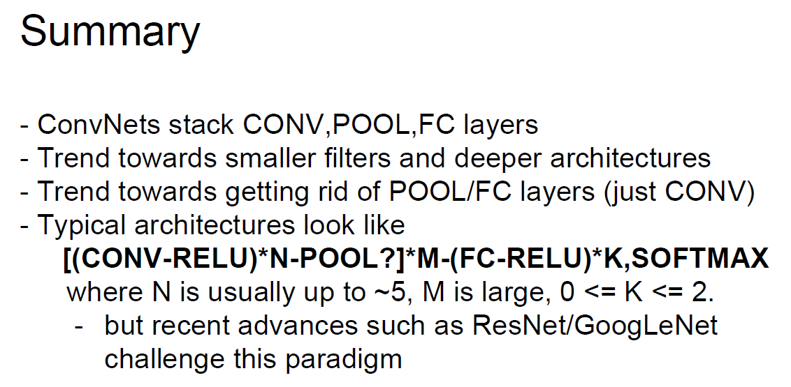
LeNet 最後三層是全連接、傳統的類神經網路。在 F6 這一層中,主要探討 activation function [9]-[14] 中的 tanh,深入的討論 [15] 放在 Appendix A中 [1],作者把這一段放在Appendix 有其道理,因為 convergence [16], [17] 需要另外討論,並不是本文小小的篇幅所能容納。

Convergence,在 RNN 中更加重要 [18]-[20],因為梯度過於陡峭或平滑都會造成難以收斂,後來發展的 Long Short-Term Memory(LSTM)[21] 有效地改善此現象。而 Dropout [22], [23] 藉著隨機丟棄神經元連結的方法,有效地改進 overfitting 的問題。若要模仿大腦運作的方式,也許可以引進 Mirror Neuron System(MNS)的概念 [24]-[28]。

-----

Questions

Q1:3 layers
Q2:Back propagation
Q3:Activation function
Q4:Convergence
Q5:Overfitting and dropout
Q6:Mirror neurons

-----

Q1:3 layers

第一個問題是:全連接層,為何要設成三層,答案是:不一定。

圖1a 的 LeNet-5 全連接層是三層。圖1b 是類似的架構。圖1c、1d 則可說是全連接層的嘗試。參考圖1e,兩層的話效能不佳,三層以上就好些,當然更多層效能更好。

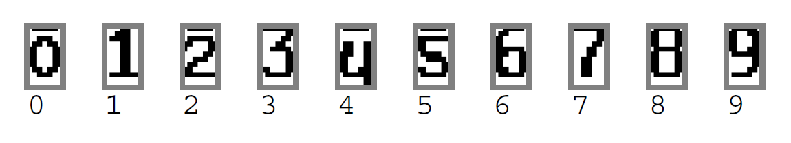
由於 LeNet-5 有多層的 convolution 與 sub-sampling layers,所以全連接層雖然只有三層,效能還是很好。輸入端這幾層的概念,來自 Fukushima,參考圖1f、1g、1h、1i。只是 Fukushima 並未導入 BP,因此效能不佳,參考圖2f,連簡單的 5 都會識別錯誤。

較完整的作法,是 convoluton + sub-sampling + BP,可以識別較複雜的數字,參考圖2a、2c。如果缺 convolution 或 BP,則只能識別較無變化的數字,如圖2d、2e。

-----

圖一:


Fig. 1a. Last 3 Layers [1]。


Fig. 1b. Convolutional parts [2]。


Fig. 1c. Full connected parts, Net-1 to Net-3 [3]。


Fig. 1d. Full connected parts, Net-4 and Net-5 [3]。


Fig. 1e. Nets, full connected parts, comparison of performance [3]。


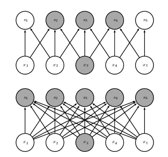
Fig. 1f. Neocognitron, simple, complex, and hypercomplex cells [4]。


Fig. 1g. Neocognitron, convolutional structures [4]。


Fig. 1h. Neocognitron, sparse connection [4]。


Fig. 1i. Neocognitron, activation function [4]。

-----

圖二:


Fig. 2a. LeNet-5, inputs [1]。


Fig. 2b. Initial parameters of the output RBFs [1]。


Fig. 2c. Zip codes [2]。


Fig. 2d. Nets, inputs [3]。


Fig. 2e. Neocognitron, inputs [4]。


Fig. 2f. Neocognitron, weak performance [4]。

-----

Q2:Back propagation

問題二,為何 Fukushima 不用 BP [7], [8],答案是,當時 BP 還不流行 [5], [6]。

"To my knowledge, the first NN-specific application of efficient BP as above was described in 1981 (Werbos, 1981, 2006). Related work was published several years later (LeCun, 1985, 1988; Parker, 1985), p. 91." [6].

Fukushima 這篇是 1983 年發表,根據上文,BP 在 1981 才正式用在 NN,以當時資訊的流通程度,嗯。所以我們大概可以說:

Fukushima + Werbos = LeCun。

-----

Q3:Activation function

F6 這一層,在論文中,重心放在為何要使用 tanh,而且是放在附錄中 [1]。圖3a 是論文用的 activation function。參考圖3b、3c,比起 sigmoid,tanh 是好一點,不過後來,其實也不能說後來,因為早在 Fukushima,就用過ReLU,參考圖1i。ReLU [12], [13] 之外,也有更新的 maxout [14]。所以究竟要簡單瞭解一下 tanh,還是要深入探討,從 fixed point [15] 挖下去,我想先不要挖比較保險。因為這牽涉到問題四,convergence 是個大問題。

"Usually, the parameters in the linear components are learned to fit the data, while the nonlinearities are pre-specified to be a logistic, tanh, rectified linear, or max-pooling function." [11].

"The rectified linear activation function (Jarrett et al., 2009; Glorot et al., 2011), which does not saturate like sigmoidal functions, has made it easier to quickly train deep neural networks by alleviating the difficulties of weight-initialization and vanishing gradients. Another recent innovation is the “maxoutactivation function, which has achieved state-of-the-art performance on multiple machine learning benchmarks (Goodfellow et al., 2013)" [11].

在 [10] 中提到 ReLU 比較好,上面的 [11] 則告訴大家,也要多注意 maxout 這個較新的 activation function。至於簡單的比較,則放在 [9]。

F6 到 F7 這一層並沒有用 tanh,而是用 RBF,參考圖3d,這跟 LeNet-5 主要想處理 ASCII 有關。經過了 ASCII 的濾波器,參考圖2b,我們可以看到圖2a 的 F6 層已經跟 ASCII 很像,這時再使用 RBF 轉到 F7 的輸出層就順理成章了。有關 RBF,之後有時間再討論。

圖四1a 跟 1b 分別是 [1] 跟 [3] 的 cost function,可看出這兩篇論文有相關性。[3] 並沒用 RBF,因為 [3] 的原始輸入已經跟 [1] 的 C5 層很接近(我猜的),所以 [3] 就直接進全連接層了。有關 cost function,之後有時間再討論。

-----

圖三:


Fig. 3a. Activation function, Atanh(Sa) [1]。


Fig. 3b. Activation function, tanh(x) [9]。


Fig. 3c. Activation function, graph of tanh(x) [9]。


Fig. 3d. RBF, Radial basis function [1]。

-----

圖四:


Fig. 4a. Cost function [1]。


Fig. 4b. Cost function [3]。

-----

Q4:Convergence

F6 這一層主要是討論 tanh 的 convergence。有種種方法可以改進 neural networks 的 convergence  [16], [17]。這個 issue 在 RNN 中更顯重要 [18]-[20],後來 Hochreiter 跟 Schmidhuber 提出 LSTM [21] 的模型來改善 RNN 不易收斂的問題。無論如何,這個問題更大、更基本,已超出本文的篇幅,以及作者現階段的能力了。

-----

Q5:Overfitting and dropout

"Large networks are also slow to use, making it difficult to deal with overfitting by combining the predictions of many different large neural nets at test time. Dropout is a technique for addressing this problem. The key idea is to randomly drop units (along with their connections) from the neural network during training. This prevents units from co-adapting too much." [23].

Convergence 是效能的議題,Overfitting 也是效能的議題。所謂 Overfitting,簡單說,就是考古題做的好,真的到考場,表現卻不佳。訓練好,測試不佳,遑論應用。

"When training with Dropout, a randomly selected subset of activations are set to zero within each layer. DropConnect instead sets a randomly selected subset of weights within the network to zero. Each unit thus receives input from a random subset of units in the previous layer." [22].

Dropout 是用來解決 overfitting 的方法之一 [23]。把 dropout 一般化,則是 dropconnect  [22]。事實上,dropout [23] 跟 maxout [14] 是一組的,藉著隨機丟棄神經元的方式簡化網路,改進效能,參考圖5。這方法已經跟真實的腦神經在使用中減少不必要的連結以強化某項功能很接近,只是,隨機?真的會好嗎?還是,不應該隨機,而是要找出某種更像大腦真實運作的方法呢?

跟 convergence一樣,overfitting 也超出本文範圍了。

-----

圖五:


Fig. 5. Dropout [23]。

-----

Q6:Mirror neurons 

我是很驚訝 dropout 這麼晚才被提出,因為腦神經科學的研究已經很久了。我才剛接觸 deep learning(DL),就想到這個點子,然後就發現 dropout 已經有人做了。我認為 mirror neurons 的概念或許有助於 DL 往真正的人工智慧,也就是 Strong AI 前進。

有關運動神經元,我也沒去找最新的研究來看,只是先就之前的論文資料庫中剪一些讀者可能會感興趣的部分,參考圖6a、6b、6c、6d。就我浮面的瞭解,目前 DL 應該是還沒有人往這方向邁進。

鏡像神經元主司模仿,「其發現始於 1992,迪⋅派勒吉諾,發現猴子的 F5 神經元,不只會在猴子本身抓香蕉時活化,也會在猴子看到其他人/猴子抓香蕉時活化。然後再經過四年,里佐拉蒂的研究團隊不斷重複檢測該實驗結果,才在 1996 年正式用“鏡像神經元"發表在 Brain 和 Cognitive Brain Research等國際知名期刊中,開啟鏡像神經元之於認知神經科學的世紀革命。」[26]。

「而人類大腦的鏡像神經系統,已知包括前運動皮質之腹側(或布洛卡區)(ventral premotor cortex)、頂葉下側小葉(inferior parietal lobule)、前扣帶迴皮質(anterior cingulated cortex)、及腦島(insula) 」[26]。

「從神經解剖學的觀點來看,被某些學者歸類為「情感型鏡像神經元系統」(affective mirror neuron system)的腦島前區與前扣帶回(anterior cingulate)裡面,確實有些較特別的神經元,伸出了長長的軸突,將前額葉、顳葉、邊緣系統緊密相連,讓它們之間的訊息傳遞更為快捷、直接,這種神經元稱為 spindle neuron(von Economo neuron)」 [28]。

「大翅鯨、大猩猩與黑猩猩跟人類一樣,在情感型鏡像神經元系統中都有 spindle neuron 作為聯繫運動、知覺、情感的樞紐。音樂與語言的相似性與相異性,在音樂學領域中已有許多討論,然而從生物演化的角度來看,這兩者都應該被納入更廣泛、更原始的「運動功能」中重新思考。從鏡像神經元的觀點來解釋音樂認知,可能還需要結合動作科學(movement science)與有關小腦的知識,此一理論才能夠趨於完備」 [28]。

-----

圖六:


Fig. 6a. Lateral view of the monkey brain showing [24]。

“In color, the motor areas of the frontal lobe and the areas of the posterior parietal cortex. For nomenclature and definition of frontal motor areas (F1–F7) and posterior parietal areas (PE, PEc, PF, PFG, PG, PF op, PG op, and Opt) see Rizzolatti et al. (1998). AI, inferior arcuate sulcus; AS, superior arcuate sulcus; C, central sulcus; L, lateral fissure; Lu, lunate sulcus; P, principal sulcus; POs, parieto-occipital sulcus; STS, superior temporal sulcus.” [24].


Fig. 6b. Mirror neuron system [25]。

“Neural mechanisms of imitation. Shown is a representation of the core circuitry for imitation on the lateral wall of the right cerebral hemisphere, together with the internal models the circuitry implements during imitation. Abbreviations: MNS, mirror neuron system; STS, superior temporal sulcus.” [25].


Fig. 6c. Neural mechanisms of imitative learning and social mirroring [25]。

“In this model, imitative learning is implemented by interactions among the core imitation circuit, the dorsolateral prefrontal cortex (BA46) and a set of areas relevant to motor preparation (PMd, pre-SMA, SPL), whereas social mirroring is implemented by the interactions among the core imitation circuit, the insula and the limbic system. Abbreviations: BA46, Brodmann area 46; MNS, mirror neuron system; PMd, dorsal premotor cortex; pre-SMA, pre-supplementary motor area; SPL, superior parietal lobule STS, superior temporal sulcus.” [25].


Fig. 6d. Mirror neuron system and music [28]。

-----

結論:

從 LeNet-5 這個 CNN 的全連接層,討論到 activation function 的 convergence,到 overfitting、dropout、以及 mirron neurons,本次提出的問題多於回答的問題。未來問題只有越來越多越難,回答只有越來越慢越辛苦。然而,每回答出一個問題,總是令人雀躍、萬分喜悅的。

大家一起加油吧!

-----

補充:看起來 DL 跟 MNS 有一起被探討,但是在 DL 圈尚未應用這個概念去開發 Nets [29]-[31]。

-----

出版說明:

2019/09/24

本篇是剛接觸深度學習時的筆記。限於當時的能力,無法進行深入的討論,不過找了一些歷史文件,還是有一些價值。人工智慧、認知科學、腦科學三者的交集被歸於智能科學,而深度學習是人工智慧的一支,所以本文也涉及了一點點腦科學的討論。

-----

References

[1] 1998_Gradient-Based Learning Applied to Document Recognition

[2] 1989_Backpropagation applied to handwritten zip code recognition

[3] 1989_Generalization and network design strategies

[4] 1983_Neocognitron, a neural network model for a mechanism of visual pattern recognition

[5] 反向傳播算法 - 維基百科,自由的百科全書
https://zh.wikipedia.org/wiki/%E5%8F%8D%E5%90%91%E4%BC%A0%E6%92%AD%E7%AE%97%E6%B3%95

[6] 2015_Deep learning in neural networks, An overview

[7] 1990_30 years of adaptive neural networks, perceptron, madaline, and backpropagation

[8] 1989_Theory of the backpropagation neural network

[9]Google軟件工程師解讀:深度學習的activation function哪家強?_幫趣網
http://bangqu.com/gpu/blog/5484

[10] 2015_Deep learning

[11] 2014_Learning activation functions to improve deep neural networks

[12] 2015_Delving deep into rectifiers, Surpassing human-level performance on imagenet classification

[13] 2010_Rectified linear units improve restricted boltzmann machines

[14] 2013_Maxout networks

[15] Fixed point (mathematics) - Wikipedia
https://en.wikipedia.org/wiki/Fixed_point_%28mathematics%29

[16] 1992_First-and second-order methods, for learning between steepest descent and Newton's method

[17] 1988_Improving the convergence of back-propagation learning with second order methods

[18] 1990_Backpropagation through time, what it does and how to do it

[19] 1994_Learning long-term dependencies with gradient descent is difficult

[20] 1996_Learning long-term dependencies is not as difficult with NARX recurrent neural networks

[21] 1997_Long short-term memory

[22] 2013_Regularization of neural networks using dropconnect

[23] 2014_Dropout, a simple way to prevent neural networks from overfitting

[24] 2004_The Mirror-Neuron System

[25] 2005_Neural mechanisms of imitation

[26] 2006_自閉症的破鏡之旅_鏡像神經元
http://beaver.ncnu.edu.tw/projects/emag/article/200704/%A6%DB%B3%AC%AFg.pdf

[27] 2006_Music and mirror neurons, from motion to 'e'motion

[28] 2008_音樂與鏡像神經元:從運動到情緒
http://1www.tnua.edu.tw/~TNUA_MUSIC/files/archive/49_5c388dc4.pdf 

[29] 2017_Is Spoken Language All-or-Nothing, Implications for Future Speech-Based Human-Machine Interaction

[30] 2016_Neural Information Processing in Cognition, We Start to Understand the Orchestra, but Where is the Conductor

[31] 2016_Motor development facilitates the prediction of others' actions through sensorimotor predictive learning

施叔青

 施叔青

2019/09/24

-----


-----

施叔青 16:54 25 天王星四宮 65 台灣人三部曲第三出版 水星天頂

Monday, September 23, 2019

AI 從頭學(一二):LeNet

AI 從頭學(一二):LeNet

2017/03/01

前言:

關於 LeNet-5,寫完這篇,我給自己打 70 分勉強及格。

-----


Fig. Net(圖片來源:Pixabay)。

-----

Summary:

LeNet-5 [1]-[2],是 Convolutional Neural Network (CNN) [3]-[8] 的基本應用。關於CNN,有網路上的投影片 [9]-[11]、論文章節 [12]-[15]、電子書章節 [16]-[18] 可供參考。

CNN 重要的計算,分別有 Convolution [19]-[20]、Activation function [21]、與 Sub-sampling [19]-[20]。有關 LeNet-CNN 的實作,可參考 Caffe [22]-[23]、TensorFlow [24]、Theano [25]-[26]、與Keras [27]。

CNN 是深度學習(目前幾乎是人工智慧的代名詞)的一支,主要,但不限於影像辨識。它的架構受到大腦視覺皮層研究的啟發 [28]-[35],由於近年來電腦軟硬體運算能力提升很多,因此蔚為風行。

-----

Hierarchy

C1 6@28x28, simple cells (edges)
S2 6@14x14
C3 16@10x10, complex cells (object parts, shapes)
S4 16@5x5
C5 (120@1x1)=8x15 (objects, topological)
F6 84=7x12 (physical)
F7 10 (abstract)

LeNet-5 共有七層,參考圖1a。在解說每層之前,先簡單介紹一下整體架構以便瞭解。

C1、C3、C5 是 convolution layer,主要是萃取影像的特徵。在生理上,「大約」可以對應到視覺皮層的 V1、V2、V4、IT 等構造,參考圖1b、1c。這個設計是受到生理學家做的實驗所啟發,在貓或猴子的初級視覺皮層置入電極,對不同方向的線條刺激,反應也有所不同,參考圖1d。

C1、C3、C5「大約」可以對應 simple cells、complex cells、以及 hypercomplex cells [32]-[34]。

S2、S4 主要都是縮小資料量。

最後 F6、F7 則是傳統的類神經網路。

Convolution 的層級不一定只有三,也可以更多。如果是三層,我們可以假定 C1 是偵測邊緣的線條,C3 偵測物體的局部,C5 偵測整個物體,參考圖1e。如果是四層,可以分成 edges、motifs、parts、objects [14] 。

-----

圖一:


Fig. 1a. LeNet-5 [1]。


Fig. 1b. Sketch of the Hmax hierarchical model of visual processing, p. 16, [35]。


Fig. 1c. The extrastriate cortex, p. 220, [30]。


Fig. 1d. Experiments of single neurones in the cat's striate cortex, p. 7, [11]。


Fig. 1e. Hierarchy of face recognition, p. 478 [16]。

-----

Q1:What do these numbers (Input: 32x32, C1: 6@28x28, S2: 6@14x14, C3: 16@10x10, S4: 16@5x5, C5: 120, F6: 84, Output: 10) mean? 
Q2:What is sparse connectivity? 
Q3:What are shared weights? 
Q4:What is zero padding?

這邊還是採取自問自答的方式進行。

-----

Q1:What do these numbers (Input: 32x32, C1: 6@28x28, S2: 6@14x14, C3: 16@10x10, S4: 16@5x5, C5: 120, F6: 84, Output: 10) mean?

-----

A0_Input: 32x32

輸入層是 32x32 pixels 的圖片,為何是 32,這在論文中解釋的很清楚。因為原始圖片的大小是 28x28。32x32 做完 5x5 filters 的 convolution 後,影像,也就是 feature maps 的大小會變成 28x28,不致於有邊緣資料訊息的損失。細節請參考圖2g 與底下 zero padding 的說明。

-----

A1_C1: 6@28x28

32x32 的原始圖片經過六個 5x5 的 edge filters 後,變成六張 28x28 的圖片,這些圖片稱為 feature maps,因為這些圖是由不同角度的線條所組成。六是一個參考值,也可以設為八,如圖2a。Filters 也可以更複雜如圖2b、2c、2d。真實的 filters 長什麼樣,可以參考圖2e。

Convolution 的運算,在一維的空間,可以想成多項式相乘。概念推到二維,就是圖片跟 filter 的 convolution,詳細的運算式,可以參考 [19]-[20]。

做完 convolution 後,緊接著是 activation function,這在圖1a並沒有標示出來,可參考圖3a。主要的 activation functions 有 sigmoid 與 ReLU,見圖3b、3c。關於 activation functions 的介紹,請參考 [21]。

這邊對 C1 做個小結:32x32 的原始圖片,經過六個 5x5 的 edge detection filters 後,變成六張 28x28 的 feature maps,然後再做 activation operation。

值得注意的是 filters 的數目、大小,都是可調整的 [25]。Activation function 的選擇,則以ReLU 為佳 [21]。

-----

圖二:


Fig. 2a. Edge filters, [8]。


Fig. 2b. Cortical filter models of the primary visual cortex, p. 2, [35]。


Fig. 2c. Divisive normalization in the primary visual cortex, p. 5, [35]。


Fig. 2d. A computer emulation of "edge detection" using retinal receptive fields [31]。


Fig. 2e. Edge detection filter, p. 7, [9]。


Fig. 2f. Complicated filter, p. 15, [9]。


Fig. 2g. Filter size, input/output size, and zero padding, p. 12, [9]。

-----

圖三:


Fig. 3a. Non-linearity, [23]。


Fig. 3b. Sigmoid function, p. 475, [16]。


Fig. 3c. ReLU function, [5]。

-----

A2_S2: 6@14x14

S2 相對 C1 簡單不少。

六張 28x28 的 feature maps 做完 subsampling 後,得到六張 14x14 的feature maps。主要目的是減少資料量以便運算。方法是每 2x2 的方塊取一點。或者取最大的一點,或者是四點平均,叫做 pooling,參考圖4a。一樣,做 max-pooling 時,方塊大小也是可以調整的 [25]。

除了減少運算量,sub-sampling 還有許多好處,譬如避免 overfitting,參考圖4b,然而最新的趨勢是增加 convolutional layers 的層數,pooling 不做,參考圖4c。Overfitting,簡單說,就是做考古題時接近滿分,真的上考場表現卻大不如預期。

-----

圖四:


Fig. 4a. Sub-sampling, p. 19, [9]。


Fig. 4b. Advantages of pooling, [5]。


Fig. 4c. Trends of ConvNets, p. 89, [11]。

-----

A3_C3: 16@10x10

六個 14x14 的 feature maps 經過 C3 後,會變成十六個 10x10 的 feature maps。

Filters 的大小還是 5x5,所以 14x14 會變成 10x10。然後十六個 feature maps 是由六個中哪些得出,參考圖五,比方說,十六個中的第一個,由六個中的第一二三個分別做完 convolution 再組成。

參考圖1e跟2f,我們可以知道這一層要把線條組成局部的圖,以數字而言就是圓圈、半圓、折線、直線、十字等等。角度不要太大,所以要連續取好幾個。希望要有點變化,兩個太少,至少要三個。然後是連四。連二加連二已經接近連六。最後是連六,十字可能就由連六獲得。這段是由現有資料推論得來。

Convolution之後,還是 activation operation。

-----

圖五:


Fig. 5. Connections between S2 and C3, p. 8, [1]。

-----

A4_S4: 16@5x5

10x10 再經過 sub-sampling 之後,變成 5x5。

-----

A5_C5: 120

這一層其實是 16@5x5,經過 5x5 的 filters 後,變成 120@1x1。120 個點,就可以跟下一層的 84 個點做一個 full connection。

為什麼是 120 呢?這邊要大膽猜測一下,因為下一層是 7x12,所以這一層取 8x15,稍微大一點,可以看成是拓樸(形狀)上的 0 到 9。下一層是實體的 0 到 9,最後一層是抽象的 0 到 9。

參考圖2f、1e,這一層所有的點組合起來應該已經不是如圖2f 的局部,而是如圖1e 的最高層,是數字的形狀了。因為已經有三層 filters 了。

-----

A6_F6: 84

84,是 7x12 的 ASCII 字元,參考論文 [1]。

-----

A7_F7: 10

A7 這一層決定輸出是 0 到 9 哪一個數字,由前一層 7x12 個點計算 Euclidean Radial
Basis Function units (RBF) 。這一段我還是不很懂,只能說需要強調的點(w大)存在(x大),或者不需要強調的點(w小)不存在(x小),則 error 小。未來若有機會再另行補充。

A0 到 A7 分別 Answer了 Q1 這七層為何要如此設計。

-----

Q2:What is sparse connectivity?

CNN在每兩層的連接,不一定要全部的點都連起來,參考圖6a、6b、6c。主要是利用 receptive fields 的特性:V1 上的 simple cells,只會對視網膜上的小塊區域的刺激有反應 [28]-[35]。V4 上的 complex cells,反應的範圍就很大。

所以 Sparse connectivity 一方面減少資料的運算,一方面有生理學的基礎,而實際的表現也很好。

-----

圖六:


Fig. 6a. Sparse connection, [25]。


Fig. 6b. Sparse connectivity, viewed from below, p. 336, [3]。


Fig. 6b. Sparse connectivity, viewed from above, p. 337, [3]。


Fig. 6c. The receptive field of the units in the deeper layers of a convolutional network is larger than the receptive field of the units in the shallow layers, p. 337, [3]。

-----

Q3:What are shared weights ?

這邊我想先抄幾段參考資料的英文,然後再用中文簡單說明。

Weights of the same color are shared—constrained to be identical [25].

In a convolutional neural net, each member of the kernel is used at every position of the input (except perhaps some of the boundary pixels, depending on the design decisions regarding the boundary) [3].

The kernel moves along (and thus shared across) the input with strides (or subsampling rate) Sr and Sc at the vertical (row) and horizontal (column) direction, respectively [18].

Here, the key idea is that if a feature detector is useful in one part of the image, it might be useful in another part as well [17].

In other words, if a motif can appear in one part of the image, it could appear anywhere, hence the idea of units at different locations sharing the same weights and detecting the same pattern in different parts of the array [14].

Shared weights 其實是緊接著 sparse connectivity 而來,一個 spacial filter 掃過整張畫面,這個 filter 的值其實是不變的,譬如,對一張畫面要萃取橫條紋,就用同一個 filter,這不是理所當然嗎?參考圖7a、7b。

與 sparse connectivity 相同,shared weights 也減少運算量。

-----

圖七:


Fig. 7a. Weights sharing, [25]。


Fig. 7b. Weights sharing: Black arrows indicate the connections that use a particular parameter in two different models, p. 338, [3]。

-----

Q4:What is zero padding?

由於 convolution 會讓圖越變越小,參考圖2g。若要避免,可以做 zero padding。也有不做 zero padding的例子  [19]。

-----

Jason Tsai:「補充一下,28x28 原圖擴展成 32x32 當作輸入是在原圖四邊補空白黑邊,稱為 zero padding,在這個辨識像這種小像素數字和英文字母的應用中,維持 C1 後仍為 28x28 的目的有二:1. 避免像素空間特徵的損失、2. 避免邊緣特徵的流失。在現在彩色大像素已事先 normalized 的圖片辨識中 zero padding 多用來微調輸入圖片大小以匹配 convolution 過程中的整數四則運算。」

-----

Conclusion:

即將寫完這篇,我想說,LeNet-5 在理解上不是太難,但設計的人可說是天才。天才不是一天造成的,也不是一個人憑空就會是天才,而是站在無數前人的努力上,更進一步。

在 LeNet 1998 之後,由於近年來硬體的運算提升,CNNs 又有更新的設計:AlexNet 2012、ZFNet 2013、GoogLeNet 2014、VGGNet 2014、ResNet 2015、DenseNet 2016 [5], [7], [11]。錯誤率繼續下降,而層數急速上升,參考圖8。而最新的趨勢,請參考圖4c。

最後,容我翻轉一下據說是貝多芬的遺言:諸君,喝采吧。喜劇已開場!

-----

圖八:


Fig. 8. Evolution of depth, p. 33, [10]。

-----

出版說明:

2019/09/23

1998 年,LeNet 奠定了 CNN 主要的架構:卷積層、池化層、全連接層。透過反向傳播法跟梯度下降法更新權重,成功辨識阿拉伯數字 0 到 9,並且應用在部分美國銀行的支票辨識系統上。

-----

References

◎ [1] 1998_Gradient-Based Learning Applied to Document Recognition

[2] Deep Learning(深度学习)学习笔记整理系列之LeNet-5卷积参数个人理解 - qiaofangjie的专栏 - 博客频道 - CSDN_NET
http://blog.csdn.net/zouxy09/article/details/8781543

◎ [3] 9 Convolutional Networks
http://www.deeplearningbook.org/contents/convnets.html 

[4] Convolutional neural network – Wikipedia
https://en.wikipedia.org/wiki/Convolutional_neural_network

◎ [5] An Intuitive Explanation of Convolutional Neural Networks – the data science blog
https://ujjwalkarn.me/2016/08/11/intuitive-explanation-convnets/

[6] Convolutional Neural Networks (CNNs) An Illustrated Explanation – XRDSXRDS
http://xrds.acm.org/blog/2016/06/convolutional-neural-networks-cnns-illustrated-explanation/

[7] CS231n Convolutional Neural Networks for Visual Recognition
http://cs231n.github.io/convolutional-networks/

[8] [DL] Convolutional Neural Network ? 不要停止思考
http://solring-blog.logdown.com/posts/302641-dl-convolutional-neural-network

[9] 6_CNN.pdf
http://classes.engr.oregonstate.edu/eecs/winter2017/cs519-006/Slides/6_CNN.pdf

[10] Convnets.pdf
http://www.cs.toronto.edu/~guerzhoy/411/lec/W06/convnets.pdf

[11] winter1516_lecture.pdf
http://cs231n.stanford.edu/slides/winter1516_lecture7.pdf

[12] 2016_Towards Bayesian Deep Learning, A Survey_3-4

[13] 2016_Deep Learning on FPGAs, Past, Present, and Future_2-3

[14] 2015_Deep learning_4-5

[15] 2009_Learning deep architectures for AI_43-45

[16] 2016_Practical Machine Learning_493-495

[17] 2015_Python Machine Learning_381-383

[18] 2015_Automatic speech recognition, a deep learning approach_288-291

[19] 2015_A guide to convolution arithmetic for deep learning

◎ [20] 2002_Tutorial on Convolutions – Torch

◎ [21] Google軟件工程師解讀:深度學習的activation function哪家強?_幫趣網
http://bangqu.com/gpu/blog/5484

[22] Caffe LeNet MNIST Tutorial
http://caffe.berkeleyvision.org/gathered/examples/mnist.html

[23] LeNet CNN 實例 MNIST 手寫數字辨識 allenlu2007
https://allenlu2007.wordpress.com/2015/11/28/mnist-database-%E6%89%8B%E5%AF%AB%E6%95%B8%E5%AD%97%E8%BE%A8%E8%AD%98/

[24] Playing with convolutions in TensorFlow — Mourad Mourafiq
http://mourafiq.com/2016/08/10/playing-with-convolutions-in-tensorflow.html

◎ [25] Theano - Convolutional Neural Networks (LeNet) — DeepLearning 0_1 documentation
http://deeplearning.net/tutorial/lenet.html

[26] 卷积神经网络 Convolutional Neural Networks (LeNet) - Maching Vision - 博客园
http://www.cnblogs.com/cvision/p/CNN.html

[27] LeNet - Convolutional Neural Network in Python - PyImageSearch
http://www.pyimagesearch.com/2016/08/01/lenet-convolutional-neural-network-in-python/

[28] 1962_Receptive fields, binocular interaction, and functional architecture in the cat’s visual cortex

[29] 1968_Receptive fields and functional architecture of monkey striate cortex

◎ [30] 2016_Ocular and visual physiology, clinical application_201-228

[31] Receptive field – Wikipedia
https://en.wikipedia.org/wiki/Receptive_field

[32] Simple cell – Wikipedia
https://en.wikipedia.org/wiki/Simple_cell

[33] Complex cell – Wikipedia
https://en.wikipedia.org/wiki/Complex_cell

[34] Hypercomplex cell – Wikipedia
https://en.wikipedia.org/wiki/Hypercomplex_cell

◎ [35] 2017_Towards a theory of computation in the visual cortex